Overview
This guide accompanies the final set of exercises for the 2021 MESA Summer School led by lecturer Ylva Goetberg and TAs Bill Wolf and Eb Farag.
About These Exercises
These lab exercises will have you exploring the topic of massive star binaries using the binary module of MESA. This page will likely fall out of date as the interface of MESA changes in its development and the hyperlinks on this page become outdated. For greatest compatibility, you should use the following versions of MESA and the SDK:
- MESA Version
- 15104
- SDK Version
- 21.4.1 (Mac or Linux)
Using a Newer Version of MESA?
Rob Farmer has created a slightly updated version of these exercises targeted at version 21.12.1. If this is your first exposure to MESA and MESA binary, you might want to start there so you don't have to account for the changes that occurred between version 15140 and 21.12.1. If you are using an even newer version… then you'll have to be brave either way!
Throughout this page, monospaced text on a black background, like this: echo "Hello, World!" represent commands you can type into your terminal and execute, while red monospaced text like this: mass_change = 1d-9 represent file names or values that you might type into a file, but not something to be executed.
Science Background
Massive stars are important for many fields of astrophysics: they are thought to have provided most of the ionizing radiation that caused cosmic reionization, their remnants merge in gravitational wave events, and they even produce the oxygen we breathe. Understanding the evolution of massive stars is therefore a key component, for example, when interpreting the radiation from distant galaxies or estimating the merger rates of neutron stars.
However, massive stars are not born alone. In fact, they spend their lives in so close of an orbit with at least one companion star that dramatic interactions are bound to happen as the stars evolve and swell. Through interaction, many solar masses of material can be exchanged between the two stars, X-rays can be produced, and the stars can even coalesce. In this lab, we will use MESA’s binary module to model a variety of interactions in massive binaries.
The Labs in Summary
We have prepared three laboratory exercises that will familiarize you with how to use the binary module to model interacting binary stars, as well as some of the difficulties you might run into in the process.
- Minilab 1
- Get familiarized with the
MESA binarymodule by modeling the evolution of a star that loses its fluffy, hydrogen-rich envelope via mass transfer to a companion star. Also experiment with changing the wind mass loss prescription. - Minilab 2
- Explore what types of supernovae to expect from envelope-stripped stars and model the prior X-ray binary phase.
- Maxilab
- Make exploratory models of binary stars that merge and further evolve the resulting merger products.
Minilab 1: Envelope Stripping in a Binary
Objectives
In this lab you will learn and practice…
- The structure of a
binarywork directory - How to model roche lobe overflow from a stellar model to a point mass
- How to implement and use a custom wind scheme for a single star
- (Optionally) How to create a custom history column and add it to a pgstar dashboard
Introduction to MESA binary
Task 0: Download Materials For both of the minilabs, we will use the same basic work directory that we will slightly modify. Additionally, for all labs, we'll use a suite of pre-computed ZAMS models. Depending on when you complete this exercise, you might find these files on the summer school dropbox, or later, at the Zenodo repository. For convenience, both the work directory and the suite of ZAMS models are available below
Starting from the tarball
-
Move the tarball/directory from your downlaods to where you'd like it to live.
mv ~/Downloads/minilab1.tar.gz PATH/WHERE/YOU/WANT/IT/ -
Navigate to the enclosing folder
cd PATH/WHERE/YOU/WANT/IT -
Untar the files
tar -xvzf minilab1.tar.gz -
Finally, navigate to the
minilab1folder within the new directory.
cd minilab1/minilab1.
Starting from a full folder download (Dropbox/Zenodo)
- Find the appropriate folder on Dropbox (during the summer school) or Zenodo (afterward) and download it.
-
Move the folder from downloads to where you'd like it to live long term.
mv ~/Downloads/minilab1 PATH/WHERE/YOU/WANT/IT/ -
Navigate to the
minilab1directory within the downloaded folder:
cd PATH/WHERE/YOU/WANT/IT/minilab1
Finally, list the files in the directory (ls) and notice the similarities and differences from a typical MESA star work directory.
MESA has a binary module, which is very similar to the star module, but has the capability to evolve two stars simultaneously while also accounting for mass exchange between them. To accommodate both stars and the binary orbit, there is one inlist for the binary orbit (inlist_project) which points to one inlist for each of the stars (inlist1, inlist2). It is also possible to evolve just one of the stars in the system, while treating the other as a point mass, which can be handy when simulating systems composed of a star and a compact object. Similar to the star module, there is a binary_history.data output file which tracks information about the binary system while there still are the history.data and profile files for the individual components in their respective LOGS1/2 folders. There is also a run_binary_extras.f90 file in the src directory, for when you need to access the two stars at the same time or interact with parameters of the binary orbit.
Click through on some of the file names below. Most that look familiar from star have similar or identical functions in binary, but in some cases, like the multiple inlists and LOGS directories, are more nuanced.
Similar to the same file in star work directories, but this inlist controls the three binary namelists (binary_job, binary_controls, and binary_pgstar). Often this points to other inlist files to separate different functionalities, like inlist_project.
Envelope Stripping with a Black Hole Companion
About a third of all massive stars are expected to lose their hydrogen-rich envelopes either via mass transfer or the successful ejection of a common envelope. Here, we start exploring envelope-stripping via Roche-lobe overflow (RLOF, mass transfer) in a binary initially composed of a 14 M⊙ star that orbits an 8 M⊙ black hole every 20 days. To speed up the models, we will model stars at the sub-solar metallicity Z = 0.006 (similar to the metallicity in the Large Magellanic Cloud).
Task 1: Prepare your Model While in the minilab1 work directory…
-
Update the initial masses and initial period of the two stars in
inlist_project. Star 1 will be the 14 M⊙ star, and star 2 will be the 8 M⊙ black hole. -
Locate the 14 M⊙ zero-age main sequence model in the
ZAMS_modelsfolder and make sure your simulation will use it to start from. -
Update
inlist_donorto reflect that this starting model uses a different metallicity than the default inMESA. - Compile and run the code.
MESA Warning: Low Resolution Runs
The process of determining the correct mass transfer rate in a binary run is an iterative process. Essentially, the solver guesses a mass transfer rate and then checks to see if the donor star has receded within its roche lobe. It then tries to find the "right" mass transfer rate to get the final radius within some tolerance of the roche lobe.
To make these runs go more quickly, we have lowered this tolerance, as well as the general spatial and temporal tolerances of the donor star model. A more science-ready exploration should investigate if these tolerances are sufficient for robust results (they likely aren't).
MESA Pro Tip: Pesky Permissions
Did you download a whole folder or a zipped folder, and then try to use an executable like ./mk or ./rn, only to be greeted by a a message like permission denied: ./mk?
Usually this means there is a file permissions error, which can arise from these ways of transmitting files. If you execute ls -l in the directory, and the lines for those executable files (like rn) don't start with -rwx, and instead have -rw- (i.e., the "x" is missing from the first four characters), you do not have permission to execute the file, which is exactly what you want to do.
The solution is simple, fortunately! Just give yourself execution priveleges on those files:
chmod +x mk
chmod +x rn
chmod +x re
Check that the permission was updated with ls -l again. If the "x" is present, you should be able to use these executables properly.
Note: some will recommend using chmod 777 instead of chmod +x, which will also work, but is overly generous with applying priveleges to all users rather than just yourself. It's not a great habit to pick up since you might apply this panacea where differential permissions really are important.
Set the masses of the two stars and their initial orbital period in inlist_project:
&binary_controls

 ! Initial conditions for the binary
   m1 = 14.0d0 ! donor mass in Msun
   m2 = 8.0d0 ! companion mass in Msun
   initial_period_in_days = 20.0d0
Select the starting model in the star_job namelist in inlist_donor. Note that you must first copy zams_14Msun.mod to the minilab1 directory from the ZAMS_models directory (or you could give a path like ../ZAMS_models/zams_14Msun.mod)
  ! Load ZAMS model
    load_saved_model = .true.
    saved_model_name = 'zams_14Msun.mod'
Finally, we must account for the reduced metallicity in the stellar model in inlist1:
&kap
  ! kap options
  ! see kap/defaults/kap.defaults
  use_Type2_opacities = .true.
Zbase = 0.006initial_z since we are loading a saved model that already has that information. However, this data is written to any saved model that is created from the inlist, so it's a good practice to also set initial_z to 0.006.
To compile, execute ./mk and to run, execute ./rn as usual.
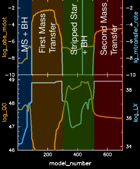
A large pgstar dashboard should pop up. Study each panel and see if you can understand what they are showing you. Can you recognize the mass transfer phase in the Hertzsprung-Russell diagram? Can you distinguish the mass transfer from wind mass loss?
Task 2: Analyze the Model At the time the simulation stops, the stellar model should be fusing helium to carbon and oxygen in its center. Identify the following characteristics for this binary stellar model. All quantities refer to the donor star unless otherwise indicated.
- Mass
- Effective Temperature
- Radius
- Peak mass transfer rate over simulation
- Final mass loss rate from donor star
- Companion (black hole) mass
- Orbital period in days
There are several places you can get this information:
- The final pgstar frame. If you closed it already, you can find all frames saved in
grid_png(or make a movie out of these! See the tip below). - Terminal output. Do note that there are two types of outputs now. One is the standard one for
star(for the donor star) and the other is for quantities relevant to the binary, which always start withbinin the upper left. - The binary history (
binary_history.data) and donor history (LOGS1/history.data) files.
You can find the following by closely studying the last pgstar frame, LOGS1/history.data and/or binary_history.data. Note that pgstar frames have been saved to the grid_png folder so you can look at them after the run.
- Mass: ≈ 5.3 M⊙
- Effective Temperature: ≈ 91,000 K
- Radius: ≈ 0.91 R⊙
- Peak mass transfer rate over simulation: ~ 10–2 M⊙
- Final mass loss rate from donor star ~ 10–6 M⊙/yr
- Companion (black hole) mass: ≈ 15 M⊙
- Orbital period in days: ≈ 38 days
As you can see, this is not a regular 5 M⊙ star! It is extremely hot and very small, since it is essentially the exposed helium core of a massive star.
MESA Pro Tip: Making pgstar Movies
The inlist_pgstar_binary inlist is instructing your model to dutifuly output pngs of pgstar frames to the folder grid_png. While you shouldn't need past frames to answer the questions in this task, you still might find it useful to create a movie out of these. Fortunately, that ability is baked in to the MESA SDK! Simply use the script images_to_movie.
images_to_movie takes a glob string and a name for an output video file. The glob string should be something like 'grid_png/grid_*.png' (the quotes are evidently important!), which can match the files you wish to use as frames. Then the output file should end in mp4 to indicate making an mp4 movie, so something like to_he_exhaustion.mp4. So putting it all together:
images_to_movie 'grid_png/grid_*.png' to_he_exhaustion.mp4
Updating the Wind Mass-Loss Scheme
The default wind mass-loss rate for stripped stars in MESA is an extrapolation of the Nugis & Lamers (2000) empirical wind mass-loss recipe created from a sample of Galactic Wolf-Rayet (WR) stars. This extrapolation reproduces relatively accurately the wind mass loss rate from the only published intermediate mass stripped star, the ≈4 M⊙ quasi-WR star in the binary HD 45166 (Groh et al., 2008). However, a recent theoretical model from Vink (2017) predicts that the wind mass loss rate from intermediate mass stripped stars should be significantly lower. This is because WR stars are so bright that radiation pressure contributes to the wind mass-loss, while it should be unimportant for intermediate mass stripped stars, which are less luminous. As a result, Vink (2017) proposed that the wind mass-loss rate from stripped stars is related to the luminosity and metallicity following the relation:
\[\log\dot{M} = -13.3 + 1.36\log\left(L/L_\odot\right) + 0.61\log\left(Z/Z_\odot\right)\]
If stellar winds are strong, they can significantly alter the stellar properties of a star, revealing deeper, chemically enriched layers. For stripped stars, the amount of hydrogen left over after mass transfer not only affects the stellar properties, but also the possibility to interact again and the supernova type (see minilab 2).
Task 3: Implement a Custom Wind Make a copy of your first work directory that you used for the first two tasks. In the new directory, implement the Vink (2017) wind mass loss rate for stripped stars with mass <10 M⊙ in the run_star_extras.f90 file and activate the other_wind hook. Note that we have prepared a function into which you can implement the new wind mass loss scheme.
So that we maintain the old work directory, which we'll need later, we need to duplicate our starter directory. First, navigate back up a level:
cd ..
And now we need to copy the whole directory to a new one and then enter it. You can pick any name for this directory, but pick something that helps you understand what's special about it. Here we'll call it minilab1_vink17:
cp -r minilab1 minilab1_vink17
cd minilab1_vink17
While not essential, you might also consider clearing out old logs, photos, and pgstar data to prevent old data from interfering with new data:
rm -f photos/*
rm -rf LOGS1
rm -f grid_png/*
Usually, to implement the other_wind hook, you need to write your own subroutine to actually compute the wind (pursuant to a particular signature found in $MESA_DIR/star/other/other_wind.f90). However, we've already done most of that for you here. Look inside src/run_star_extras.f90 and see if you can find the routine that [mostly] computes the wind for our stellar model.
Once you've found the routine, edit it so that the Vink (2017) routine fires when the model has
- a mass less than 10 M⊙ AND
- a surface hydrogen fraction less than 0.40
contains keyword) to actually evaluate the wind mass loss rate. You might emulate this organization and create your own internal subroutine whose sole job is to set its lone input w to the mass loss rate described in the equation above, and then calling it in the if/else block under the correct circumstances.
You should start to see the modified wind in use sometime around star 1's model number 1028 (equivalently, binary model number 159). Consider adding a write statement to confirm that it is being called at this time.
Once you have updated the implementation of the wind routine, you need to do two things to have it actually get called:
- Point
s% other_windto the routine that should set the wind (inextras_controlswithinrun_star_extras.f90). - Ensure that a line (not shown here) is added to the
controlsnamelist of star 1 that tells it to use the other wind hook.
The name of the subroutine we provided to do this is weak_wind_stripped_stars. To have this be called by the other_wind hook, we need to point to it in the extras_controls subroutine in run_star_extras.f90:
      subroutine extras_controls(id, ierr)
         integer, intent(in) :: id
         integer, intent(out) :: ierr
         type (star_info), pointer :: s

         ierr = 0
         call star_ptr(id, s, ierr)
         if (ierr /= 0) return

         s% extras_startup => extras_startup
         s% extras_start_step => extras_start_step
         s% extras_check_model => extras_check_model
         s% extras_finish_step => extras_finish_step
         s% extras_after_evolve => extras_after_evolve
         s% how_many_extra_history_columns => how_many_extra_history_columns
         s% data_for_extra_history_columns => data_for_extra_history_columns
         s% how_many_extra_profile_columns => how_many_extra_profile_columns
         s% data_for_extra_profile_columns => data_for_extra_profile_columns

         ! THIS IS THE IMPORTANT BIT (earlier lines should already exist)
         s% other_wind => weak_wind_stripped_stars
      end subroutine extras_controls
But now we need to update weak_wind_stripped_stars to reflect the changes we want to make. Here's the part that decides which wind routine to use:
         ! Call the wind functions
         ! Hot and hydrogen rich stars (main-sequence stars)
         if ((Tsurf >= 1.0d4) .and. (Xsurf >= 0.4)) then
            call eval_Vink_wind(w)
         ! Hot and hydrogen poor stars
         else if ((Tsurf >= 1.0d4) .and. (Xsurf < 0.4)) then
            call eval_Nugis_Lamers_wind(w)
         ! Cool stars
         else
            call eval_de_Jager_wind(w)
         end if
We want to add an extra check to the else if block to see if the mass is less than some limiting value. If it is, we want to call a new subroutine that implements the above wind law:
         ! Call the wind functions
         ! Hot and hydrogen rich stars (main-sequence stars)
         if ((Tsurf >= 1.0d4) .and. (Xsurf >= 0.4)) then
            call eval_Vink_wind(w)
         ! Hot and hydrogen poor stars
         else if ((Tsurf >= 1.0d4) .and. (Xsurf < 0.4)) then
            if (Msurf <= Mlim) then
               call eval_Vink17_wind(w)
            else
               call eval_Nugis_Lamers_wind(w)
            end if
         ! Cool stars
         else
            call eval_de_Jager_wind(w)
         end if
We've introduced two new entities here. First is a real variable, Mlim that we need to define as 10 M⊙. First we declare it by tacking it on to the end of an existing declaration line:
real(dp) :: Tlim, Rlim, Zsurf, log10w, Ysurf, Xsurf, Mlim… and then we set its value where similar variables are set:
         ! Solar metallicity
         Zsun = 0.0134
         ! Limits
         Tlim = 1.5d4
         Rlim = 1.5*Rsun
         Mlim = 10d0 * Msun !!! the new bits; 10 solar masses
The second, and more interesting addition is the eval_Vink17_wind subroutine, which must be defined. Following a style similar to eval_de_Jager_wind, we get the following:
        ! Vink (2017) wind for low-mass stripped stars
        subroutine eval_Vink17_wind(w)
           real(dp), intent(out) :: w
           real(dp) :: log10w
           include 'formats'
           write(*,*) "Calling magic wind routine!"
           log10w = -13.3d0 + 1.36d0 * log10(Lsurf / Lsun) + &
                     0.61d0 * log10(Zsurf / Zsun)
           w = exp10(log10w)
        end subroutine eval_Vink17_wind
We can place this anywhere between the contains and end subroutine weak_wind_stripped_stars statements.
But there is one last part! We need to turn the wind on in the inlist, as well. So somewhere in the controls namelist of inlist_donor, we need to add the following:
use_other_wind = .true.AND/OR
hot_wind_scheme = 'other'
For your own sanity, you should probably put this in the WIND MASS LOSS section of the inlist. While not necessary to make this work, you should also comment out or delete the other hot and cold wind scheme controls so that you aren't confused about which wind is actually active (an other_wind scheme always takes precedence when it is activated).
Task 4: Compare Models Explore how the properties of the stripped star changed since you updated the wind scheme. Look at the same quantities we looked at in Task 2:
- Mass
- Effective Temperature
- Radius
- Peak mass transfer rate over simulation
- Final mass loss rate from donor star
- Companion (black hole) mass
- Orbital period in days
You can find the following by closely studying the last pgstar frame, LOGS1/history.data and/or binary_history.data. Note that pgstar frames have been saved to the grid_png folder so you can look at them after the run.
- Mass: ≈ 5.6 M⊙
- Effective Temperature: ≈ 76,000 K
- Radius: ≈ 1.38 R⊙
- Peak mass transfer rate over simulation: ~ 10–2 M⊙
- Final mass loss rate from donor star ~ 10–7 M⊙/yr
- Companion (black hole) mass: ≈ 15 M⊙
- Orbital period in days: ≈ 37 days
As you can see, the weaker wind for stripped stars significantly alters the effective temperature and radius of the star. This is because less hydrogen is lost via winds and since hydrogen is "fluffier" than helium, the star can be larger and therfore also a little cooler.
BONUS: Ionizing Radiation
Because stripped stars reach extremely high surface temperatures, they emit very energetic radiation. In fact, the majority of their emitted radiation is ionizing. To accurately compute the emission rate of ionizing photons, spectral models that match the properties of the stripped stars are necessary. However, the hydrogen-ionizing emission rate from intermediate mass stripped stars is quite well approximated by a blackbody radiation curve.
Bonus Task 5: Track Ionizing Radiation In the text file Q0_function.txt in the work directory, there is a function that calculates the emission rate of H-ionizing photons, Q0. Copy this function and place it in the correct place in the run_star_extras.f90 file so that you can add log(Q0) as an output in the history.data file. Make sure to call the new column log_Q0. Before compiling and running the model, un-comment the fourth panel in the pgstar window (tip: search for EDIT HERE) so that you can see the evolution of the emission rate of H-ionizing photons. It is also advantageous to set the minimum of the y-axis to 46.
Since you'll want the code in Q0_function.txt when calculating the values extra history columns, we'll want them handy inside the data_for_extra_history_columns subroutine. You can just paste the contents of the file at the bottom of the subroutine, but be sure to add a contains statement before you paste those contents.
With the code handy, you can then set the name of the new column and the value within the definition of data_for_extra_columns (before the contains statement). Setting the name is as simple as assigning names(1) to the proper string. Setting the value is more interesting, since the calculate_Q0 subroutine takes in a variable and sets its value to the log of Q0. So you won't simply do something like vals(1) = calculate_Q0. Instead, you'll need to call the subroutine with an input of vals(1).
Finally, even if you've defined the name and value of the new history column properly, it won't work until you update the value set in how many_extra_history_columns. Update this value to 1.
Look inside inlist_pgstar_binary and search for EDIT HERE. You need only make changes to the next two lines (set the name of the y-value to be plotted, and also update the minimum value on that axis). Leave the third line for now; we might get to it in the next minilab.
To create the new column in the history file, we'll need to edit the how_many_extra_history_columns function:
      integer function how_many_extra_history_columns(id)
         integer, intent(in) :: id
         integer :: ierr
         type (star_info), pointer :: s
         ierr = 0
         call star_ptr(id, s, ierr)
         if (ierr /= 0) return
         how_many_extra_history_columns = 1
      end function how_many_extra_history_columns
(The only change from the original code is the second-to-last line being set to 1 instead of 0.)
To set the name and value of the new column, you need to edit the subroutine data_for_extra_history_columns. You only need to add the two lines that set names(1) and vals(1):
      subroutine data_for_extra_history_columns(id, n, names, vals, ierr)
         integer, intent(in) :: id, n
         character (len=maxlen_history_column_name) :: names(n)
         real(dp) :: vals(n)
         integer, intent(out) :: ierr
         type (star_info), pointer :: s
         ierr = 0
         call star_ptr(id, s, ierr)
         if (ierr /= 0) return

         ! note: do NOT add the extras names to history_columns.list
         ! the history_columns.list is only for the built-in history column options.
         ! it must not include the new column names you are adding here.

         ! Add the emission rate of H-ionizing photons to the history file
         names(1) = 'log_Q0'
         call calculate_Q0(vals(1))

         contains

         ! below is just the contents of Q0_function.txt
         subroutine calculate_Q0(log10_Q0)
            ! contents omitted for brevity
         end subroutine calculate_Q0

         pure function integrate(x, y) result(r)
            ! contents omitted for brevity
         end function

      end subroutine data_for_extra_history_columns
Finally, we need to plot this quantity in the pgstar dashboard. Edit these lines in inlist_pgstar_binary:
      ! The fourth panel
      ! ! ! ! EDIT HERE ! ! ! ! ! ! !
      History_Panels1_yaxis_name(4) = '' !'log_Q0'   ! Extra exercise, minilab 1
      !History_Panels1_ymin(4) = 46  ! Extra exercise, minilab 1
to this:
      ! The fourth panel
      ! ! ! ! EDIT HERE ! ! ! ! ! ! !
      History_Panels1_yaxis_name(4) = 'log_Q0'   ! Extra exercise, minilab 1
      History_Panels1_ymin(4) = 46  ! Extra exercise, minilab 1
OB-type stars are thought to provide most of the ionizing radiation in a stellar population. Let's compare our model to published spectral models of main sequence OB stars. Below is a subset of a table taken from Smith et al. 2002 (see the full dataset in Table 1 of that paper) that shows how the emission rates of hydrogen-ionizing (Q0) photons vary with the spectral type of stellar models.
| Spectral Type | Teff (kK) | R* (R⊙) | logQ0 |
|---|---|---|---|
| O3V | 50.0 | 9.8 | 49.5 |
| O4V | 45.7 | 10.4 | 49.4 |
| O5V | 42.6 | 10.5 | 49.2 |
| O7V | 40.0 | 10.6 | 49.0 |
| O7.5V | 37.2 | 10.5 | 48.8 |
| O8V | 34.6 | 10.5 | 48.4 |
| O9V | 32.3 | 10.1 | 47.9 |
| B0V | 30.2 | 9.5 | 47.3 |
| B0.5V | 28.1 | 8.6 | 46.8 |
| B1V | 26.3 | 8.1 | 46.4 |
| B1.5V | 25.0 | 7.1 | 46.1 |
Bonus Task 6: Compare to Main Sequence Models Look at Table 1 and decide which main sequence stellar model has the most similar rate of H-ionizing photons as your stripped star? After making this comparison based on Q0 alone, compare how the stellar radius and effective temperature of the stripped model compares with the main sequence stellar model with the most similar Q0.
You should find (e.g. in the last pgstar snapshot) that log10Q0 ended a little above 48.6. Looking at the table above, that means that our stripped stellar model is most similar to an O7.5V star (log10Q0 = 48.8 in the table above).
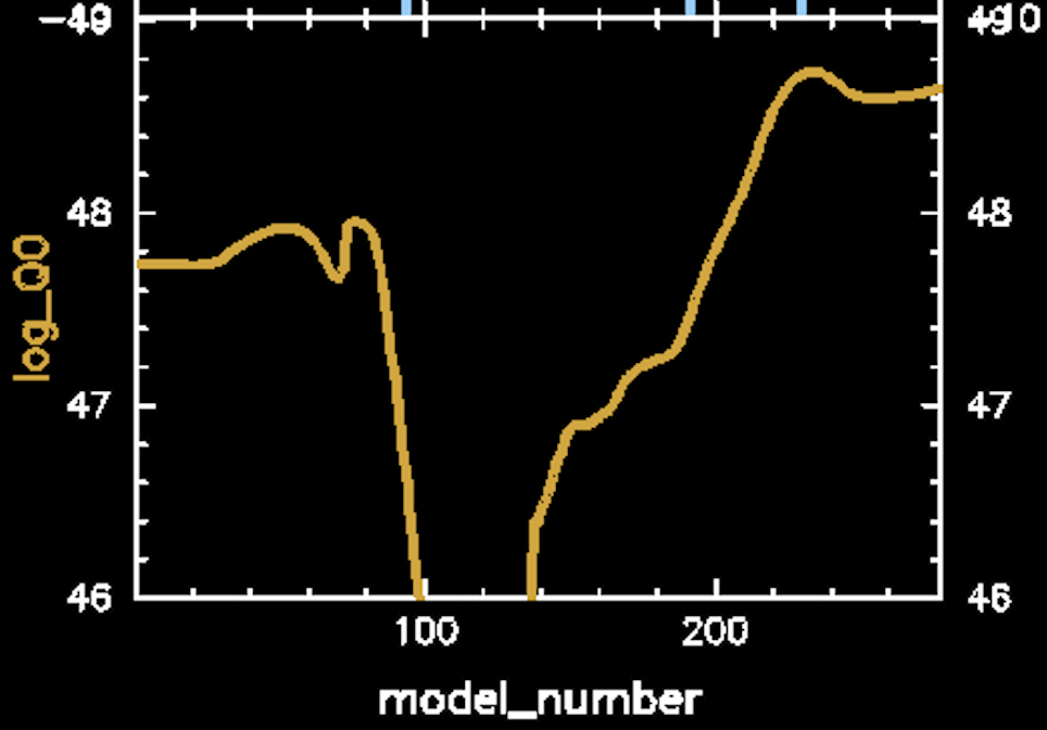
An 07.5V type stars are massive main sequence stars with masses around 20 M⊙. Note that the effective temperature of our model is roughly 40,000 K higher than its ZAMS counterpart, but its radius is about an order of magnitude smaller. This makes sense, as our smaller star must be more luminous and/or have a harder spectrum to produce the same amount of H-ionizing photons per unit time.
Minilab 2: Stripped-envelope Supernova Progenitors
Even though only one intermediate mass stripped star has been published, many supernovae thought to result from the collapse of stripped stars have been identified. These stripped-envelope supernovae constitute about a third of all core-collapse supernovae and are, unsurprisingly, hydrogen-poor (Smith et al., 2011, Graur et al., 2017a, Graur et al., 2017b).
Objectives
In this lab you will learn and practice how to…
-
Adjust stopping conditions and data reported to the terminal by
MESA starto try to produce stripped-envelope supernova progenitor models, - Perform a parameter-space study to charaterize the likelihood of observability of stripped-envelope supernova progenitors in surveys,
-
(Optionally) Use controls in the
binaryto more accurately model the mass transfer rate onto the black hole companion, and -
(Optionally) Use
run_binary_extras.f90to track a new quantity that relies on properties of the binary rather than just a single star.
Stripped-envelope Supernovae
There are three main classes of stripped-envelope supernovae, distinguished by how much hydrogen or helium they contain. Following Hachinger et al. (2012), we make the following distinctions:
- Type IIb
- Hydrogen-poor (> 0.03 M⊙), helium-rich
- Type Ib
- Hydrogen-free (< 0.02 M⊙), helium-rich (> 0.14 M⊙)
- Type Ic
- Hydrogen-free (< 0.02 M⊙), helium-free (< 0.06 M⊙)
As this list shows, the amount of leftover hydrogen at explosion is an important determinant for the supernova type. In this lab, we will explore how much hydrogen is left on the surface of stripped stars and what its effect is, not the least for what supernova the star produces.
Task 1: Prepare a Progenitor
- Navigate back to the original work directory from minilab 1 (before we updated the mass loss scheme).
- Change the stopping condition to core carbon-depletion, which we will approximate as when the central mass fraction of 12C drops below 10–2. This isn't technically "right before" core collapse, but we don't anticipate the outer regions of the star changing substantially between this time and core collapse.
- Identify and implement the inlist controls that will print the total masses of 1H and 4He in the star to the terminal with each time step. Alternatively, edit the text summary in the pgstar window to include these two pieces of data. We'll use this data to predict which type of supernova the stripped star would produce.
- Restart (i.e., do not start a new run) your model from where it stopped last (this saves a lot of time by skipping the main sequence and helium depletion).
There should already a stopping condition present for when central helium falls below 0.20. You need only update the isotope and the threshold.
Note: If we were to do a full run rather than a restart, this might pose a problem, because the initial carbon mass fraction would already be below this threshold (it hasn't yet been produced via triple alpha reactions). We would instead need to stop at some point after helium burning has begun and then change the stopping condition (essentially what we've done here) or create a clever stopping condition in run_star_extras.f90.
Can't find the inlist controls? They are in the controls namelist (and thus documented in $MESA_DIR/star/defaults/controls.defaults). Search for the word "trace" and see if you can figure out how to use them. You'll need to add three lines total to your controls namelist. You may also need to look in history_columns.list to see which quantities can be tracked.
You can restart from the last saved photo by simply executing ./re. If instead you know the specific photo you want to restart from, you can execute something like ./re PHOTO_FILE_NAME, where PHOTO_FILE_NAME is something like x850 (you can see all photos in the photos folder).
First, as a reminder, we wanted to be in the original working directory. If you came to this from the previous minilab, your session was probably in the altered version, so you'd need to execute cd ../minilab1.
The stopping condition can simply be adapted from the existing one (of reduced helium mass fraction). You should have something like the following in inlist_donor:
  ! Central abundance limit
    xa_central_lower_limit_species(1) = 'c12'
    xa_central_lower_limit(1) = 1d-2
And to track the values on the terminal, we would add the following lines to the controls namelist, also in inlist_donor:
  ! track the total masses of h1 and he4
    num_trace_history_values = 2
    trace_history_value_name(1) = 'total_mass_h1'
    trace_history_value_name(2) = 'total_mass_he4'
These lines weren't present at all before. Note that we need to first indicate the number of columns to be traced (the first line), and then we need to provide the names of the columns as they would appear in that model's history.data. Fortunately, we were already recording these two values, but if we tried to track the total mass of 12C, we would need to edit history_columns.list first.
To restart from the last photo (which should be where we left off from minilab 1), we can simply execute ./re. But, if you wanted to specify the particular photo, you could do something like ./re x278.
Task 2: Supernova Taxonomy Using the final total masses of 1H and 4He in the carbon-depleted model and the classification given above, which type of supernova do you think will result from this progenitor?
Try Again
A type IIb supernova progenitor should have at least 0.03 M⊙ of hydrogen, while this stripped model (without the Vink 17 wind scheme) should only have retained around 10–8 M⊙ of hydrogen. Check what the final total masses of 1H and 4He were in your model and try again.
Correct
Excellent. You should have found a final total mass of 1H of around 8.5 × 10⁻⁹ M⊙, which firmly puts us in type Ibc territory. However, it is still helium rich, with about 1.4 M⊙ of 4He, so it is a Type Ib supernova progenitor.
Try Again
A type Ic supernova progenitor is thought to have less than 0.06 M⊙ of 4He left, while this model should still contain around 1.4 M⊙. Check what the final mass of 1H was to determine if this is a type IIb or type Ib supernova progenitor.
Task 3: Back to Weaker Winds Perform task 1 again, but in the work directory with the updated weaker wind scheme implemented. Update your inlist(s) in the same way you did for the original work directory (see the task 1 solution for guidance). Again, restart the run rather than starting it from the beginning.
This model should enter a second phase of mass transfer. You do not need to follow it to completion, as it will be quite slow. Instead, stop the model once it is in this second phase of mass transfer and not undergoing rapid changes.
First, as a reminder, we wanted to be in the modified working directory (with the Vink (2017) wind scheme). If you came to this from the previous task, your session was probably in the original version, so you'd need to execute cd ../minilab1_vink17, though you may have called the working directory something else in minilab 1.
The stopping condition can simply be adapted from the existing one (of reduced helium mass fraction). You should have something like the following in inlist_donor:
  ! Central abundance limit
    xa_central_lower_limit_species(1) = 'c12'
    xa_central_lower_limit(1) = 1d-2
And to track the values on the terminal, we would add the following lines to the controls namelist, also in inlist_donor:
  ! track the total masses of h1 and he4
    num_trace_history_values = 2
    trace_history_value_name(1) = 'total_mass_h1'
    trace_history_value_name(2) = 'total_mass_he4'
These lines weren't present at all before. Note that we need to first indicate the number of columns to be traced (the first line), and then we need to provide the names of the columns as they would appear in that model's history.data. Fortunately, we were already recording these two values, but if we tried to track the total mass of 12C, we would need to edit history_columns.list first.
To restart from the last photo (which should be where we left off from minilab 1), we can simply execute ./re. But, if you wanted to specify the particular photo, you could do something like ./re x279.
Though we specified a stopping condition of carbon depletion, we probably won't get there in a reasonable time. The model should enter a new phase of mass transfer, and time steps will drop down to the single digits in years. This will probably happen within 200 or so timesteps from restarting, at which point you can kill off the run with ctrl-c.
Why can we stop the run even before getting to carbon depletion? Well, even though mass is being lost from the star rather rapidly, it has very little time left to live due to the low energy content in the remaining nuclear fuel. Therefore, its surface properties will not change significantly once the star has entered its second phase of mass transfer. If you have the time, go ahead and leave this model running all the way to carbon depletion; you'll find it won't change things much.
Task 4: Supernova Taxonomy revisited Using the final total masses of 1H and 4He in the Vink (2017) wind scheme model and the classification given above, which type of supernova do you think will result from this progenitor?
Correct
Nice! Regardless of when you stop the simulation, you should have more than 0.03 M⊙ of 1H left on the star (but not much more, so it won't be a standard IIp supernova), which places this firmly in the IIb progenitor scenario. Even if you run the star to carbon depletion, it will still have 0.04 M⊙ of hydrogen remaining.
Try Again
Double check your final 1H and 4He masses. In order to be a type Ib progenitor, we need less than 0.02 M⊙ of 1H and greater than 0.14 M⊙ of 4He left.
Try Again
A type Ic supernova progenitor is thought to have less than 0.06 M⊙ of 4He left, while this model should still contain around 1.7 M⊙. Check what the final mass of 1H was to determine if this is a type IIb or type Ib supernova progenitor.
Bonus Task 5: What About Type Ic Supernovae? If the second phase of mass transfer initiated during the helium shell burning of the stripped star does not last long enough for a significant amount of helium to be stripped off, how can type Ic supernovae be created?
There are at least two possible pathways:
- They can come from single stars with very strong stellar winds (WC stars).
- Low-mass versions can be created if mass transfer starts earlier for the stripped star, maybe during the central helium burning phase. This can occur if the star is stripped via common-envelope ejection. Then the post-interaction orbital period can be so short that the stripped star fills its tiny Roche lobe during central helium burning.
Supernova Progenitors
To identify what type of star is responsible for a certain type of supernova, archival images of the progenitor can sometimes be found. If the progenitor can be found, it is brighter than the magnitude limit of the observations. iPTF13bvn was a stripped envelope supernova for which the progenitor was detected (Cao et al., 2013). It was found to have V-band magnitude of ≈25 and the host galaxy is located at ≈25 Mpc distance.
MESA can provide decent estimates for the absolute magnitudes of a large number of stars using a grid of synthetic spectra (Lejeune et al., 1998). However, as you have discovered, stripped stars are not standard stars and are therefore not part of standard spectral libraries.
Task 6: Detection Distance Assuming that the model you just created is a good representation of a supernova progenitor, to what maximum distance would it be detectable if available images were limited to the magnitude V < 25 mag?
-
Identify the panel in the pgstar dashboard that shows the evolution of the absolute V-band magnitude. Can you see where
MESAis unable to compute a realistic magnitude? No need to re-run your model. You can simply locate the last frame ingrid_png. - Use the V-band history panel in the pgstar dashboard to find the final V-magnitude of your progenitor model (still in the Vink 2017 wind scheme model).
- Using the relation between distance, apparent magnitude, and absolute magnitude, \[M_V = m_V - 5\log_{10}\left(\frac{d}{1\,\mathrm{pc}}\right) + 5,\] where MV is the absolte V-band magnitude, mV is the apparent V-band magnitude, and d is the distance, compute the furthest distance away that presupernova imaging could detect this progenitor. Assume available imaging is limited to mV < 25.
The panel of interest is in the lower right of the dashboard. It's below the HR diagram, but to the left of the history panels.
From around model 230 to model 330, the magnitude becomes undefined and we see the vertical lines. This happens a few times afterwards, too. The star of course has a well-behaved V-band magnitude at these times, but due to its extreme nature, we have "fallen off the tables" that MESA uses to estimate the magnitudes from effective temperature, luminosity, metallicity, etc.
At the end of the evolution, though, we do have a V-band magnitude of approximately –6.75. If we set MV to this value and assume mV = 25 and plug these into the relation above and solve for distance, we find it is about 22 Mpc.
Thus, if this star had been in the same galaxy as iPTF13bvn, it would not have been detected in presupernova imaging because that galaxy is too distant (at about 25 Mpc).
The brightness in the V-band of the supernova progenitor is not only determined by the distance, but also by the temperature of the star -- a cooler star emits a larger fraction of its photons in the optical band compared to a hotter star. Since your stripped star model dies during mass transfer, the Roche radius and therefore also the orbital period determines how large and cool the stripped star will be at core-collapse.
Task 7: Varying Parameters Now let's do a parameter-space study to see how the supernova type varies with mass and initial orbital period.
- Make a copy of your latest run directory (with the custom wind routine) and prepare it for modeling a different stripped star. Claim a combination of stellar masses (M1, M2) and initial orbital period in the google sheet (tab "Ylva - Minilab 2") by entering your name or some other identifier in the top table. Don't forget to find the new ZAMS model and load it in your inlist.
- The stopping condition for central carbon depletion will no longer work because of the initial composition of the star. You can remove it or stop at helium depletion and restart as previously. In either case, manually stop the run once it is in the second phase of mass transfer.
- Run your model and report the absolute V-band magnitude of the donor star, the final total hydrogen mass in the model, and your supernova type prediction once it enters its second phase of mass transfer in the lower tables of the google sheet.
BONUS: High-mass X-ray Binaries
We have completely forgotten that the companion is a black hole!
Black holes cannot accrete at infinite rates. Rather, their mass accretion rates are thought to be limited by the so-called Eddington accretion rate. When the accretion rate reaches the Eddington accretion rate, the radiation pressure produced by the accretion is so strong that it can prevent accretion.
The black hole is also moving through stellar wind material as it orbits its companion star. Therefore, the black hole can accrete material also when the stars are detached and mass transfer is not ongoing.
Bonus Task 8: Updating Black Hole Accretion Search $MESA_DIR/binary/defaults/binary_controls.defaults for an inlist options to accomplish the following and implement them in inlist_project in your working directory from Tasks 3–5 (before the parameter space study):
- Limit accretion onto the black hole by the Eddington accretion rate.
-
Activate accretion of the wind from the donor. Limit this accretion to a maximum of 10% of the stellar wind mass loss (this number is not based in any rigorous reasoning). Note that in addition to the control you [hopefully] found, we also have to set
use_radiation_corrected_transfer_rate = .false.ininlist_projectto make sure that 10% of the wind mass is accreted. - Remove the stopping condition based on core composition.
We will be stopping the simulation "by hand" once it has entered the second mass transfer phase, so we don't need a stopping condition, and the carbon-depletion one will trigger instantaneously on the ZAMS model.
Don't start the model yet (we'll get there).
The name of the control is limit_retention_by_mdot_edd. From $MESA_DIR/binary/defaults/binary_controls.defaults:
! limit_retention_by_mdot_edd
! ~~~~~~~~~~~~~~~~~~~~~~~~~~~

! Limit accretion using ``mdot_edd``. The current implementation is intended for use with
! black hole accretors, as in e.g. Podsiadlowski, Rappaport & Han (2003), MNRAS, 341, 385.
! For other accretors ``mdot_edd`` should be set with ``use_this_for_mdot_edd``, the hook
! ``use_other_mdot_edd``, or by appropriately setting ``use_this_for_mdot_edd_eta``.
! Note: MESA versions equal or lower than 8118 used eta=1 and did not correct
! the accreted mass for the energy lost by radiation.

! If accreted material radiates an amount of energy equal to ``L=eta*mtransfer_rate*clight**2``,
! then accretion is assumed to be limited to the Eddington luminosity,

! ::

!     Ledd = 4*pi*cgrav*Mbh*clight/kappa

! which results in the Eddington mass-accretion rate

! ::

!     mdot_edd = 4*pi*cgrav*Mbh/(kappa*clight*eta)

! the efficiency eta is determined by the properties of the last stable circular orbit,
! and for a BH with no initial spin it can be expressed in terms of the initial BH mass Mbh0
! and the current BH mass,

! ::

!     eta = 1-sqrt(1-(Mbh/(3*Mbh0))**2)

! for Mbh < sqrt(6) Mbh0. For BHs with initial spins different from zero, an effective
! Mbh0 can be computed, corresponding to the mass the black hole would have needed to
! have with zero spin to reach the current mass and spin.

! ::

    limit_retention_by_mdot_edd = .false.
The name of the controls are do_wind_mass_transfer_1/2 and max_wind_transfer_fraction_1/2. From $MESA_DIR/binary/defaults/binary_controls.defaults:
! Wind mass accretion
! ___________________


! do_wind_mass_transfer_*
! ~~~~~~~~~~~~~~~~~~~~~~~

! transfer part of the mass lost due to stellar winds from the mass losing
! component to its companion. Using the Bondi-Hoyle mechanism.
! "\_1" refers to first star, "\_2" to the second one.

! ::

    do_wind_mass_transfer_1 = .false.
    do_wind_mass_transfer_2 = .false.
and
! max_wind_transfer_fraction_*
! ~~~~~~~~~~~~~~~~~~~~~~~~~~~~

! Upper limit on the wind transfer fraction for star *
! "\_1" refers to first star, "\_2" to the second one.

! ::

    max_wind_transfer_fraction_1 = 0.5d0
    max_wind_transfer_fraction_2 = 0.5d0
You will still need to figure out which versions of these (1 or 2) to use and set their values accordingly.
The following lines should be added to the &binary_controls namelist in inlist_project:
   limit_retention_by_mdot_edd = .true.
   use_radiation_corrected_transfer_rate = .false.
and
   do_wind_mass_transfer_1 = .true.
   max_wind_transfer_fraction_1 = 0.1d0
To remove the stopping condition, comment out in inlist_donor:
  ! Central abundance limit
  !  xa_central_lower_limit_species(1) = 'c12'
  !  xa_central_lower_limit(1) = 1d-2
As the black hole accretes material, it emits X-rays. In our model, we have the opportunity to explore different stages of the life of a high mass X-ray binary (HMXB): accompanied by a main sequence star, a stripped star, and detached and semi-detached. First, let’s just implement an approximation for how high the X-ray luminosity from the system is.
The X-ray luminosity, LX can be approximated by the function \[L_X = \epsilon\frac{GM_{\rm BH}\dot{M}_{\rm acc}}{R_{\rm acc}},\] where MBH is the mass of the black hole, Ṁacc is the accretion rate, Racc is the radius at which the accretion occurs, and 𝜖 describes how efficiently the conversion from accretion to luminosity is. For black holes, we can assume that accretion occurs at Racc = 3RSchwarzschild, where RSchwarzschild = 2GMBH/c2.
Bonus Task 9: Tracking X-ray Luminosity
-
Following the simplified calculation for X-ray luminosity above, and assuming that 𝜖 = 0.1, write a function in
run_binary_extras.f90that adds a new column calledlog_LXto thebinary_history.datafile. - Un-comment the X-ray luminosity in the pgstar window so you can follow the X-ray emission rate with time (similar to Bonus Task 5 from minilab 1).
-
Wipe out the contents of
grid_png, and then compile and run your model from the ZAMS to the second mass transfer phase.
The process for adding a history column in run_binary_extras.f90 is nearly identical to the way it is done in run_star_extras.f90. The main difference is that you need to use the binary_info object rather than the star_info object.
Just as you can find components of the star_info object in $MESA_DIR/star_data/public/star_data.inc, the analagous location in binary is $MESA_DIR/binary/public/binary_data.inc.
In here, there are objects that record the mass of each component star as well as the accretion rate onto each component star (that one is probably the harder one to identify). These are the only two you will need to compute the X-ray luminosity. Note that many members of this structure are actually arrays with two elements. Element 1 is associated with star 1, and element 2 is associated with star 2.
Though you don't need it for this exercise, you can also just get at each star's star_info object with the s1 and s2 members of the binary_info object. So for instance, if b is initiated as a binary_info object (it's conventional to use "b" for this rather than "s"), you could get at star 1's luminosity via b% s1% photosphere_L. This isn't much help when star 2 is just a point mass, though, since it doesn't have an associated star_info structure!
To add the history column, we only need to edit one function, how_many_extra_binary_history_columns:
      integer function how_many_extra_binary_history_columns(binary_id)
         use binary_def, only: binary_info
         integer, intent(in) :: binary_id
         how_many_extra_binary_history_columns = 1
      end function how_many_extra_binary_history_columns
and one subrotune, data_for_extra_binary_history_columns
      subroutine data_for_extra_binary_history_columns(binary_id, n, names, vals, ierr)
         type (binary_info), pointer :: b
         integer, intent(in) :: binary_id
         integer, intent(in) :: n
         character (len=maxlen_binary_history_column_name) :: names(n)
         real(dp) :: vals(n)
         integer, intent(out) :: ierr
         ierr = 0
         call binary_ptr(binary_id, b, ierr)
         if (ierr /= 0) then
            write(*,*) 'failed in binary_ptr'
            return
         end if

         names(1) = 'log_LX'
         call set_log_LX(vals(1))

         contains

         subroutine set_log_LX(log_L_X)
             implicit none
             real(dp) :: log_L_X, epsilon, M_BH, mdot_acc, R_acc, R_sch
             epsilon = 1d-1
             M_BH = b% m(2)
             mdot_acc = b% component_mdot(2)
             R_sch = 2 * standard_cgrav * M_BH / (clight * clight)
             R_acc = 3 * R_sch
             log_L_X = safe_log10(epsilon * standard_cgrav * M_BH * mdot_acc / R_acc)
         end subroutine set_log_LX

      end subroutine data_for_extra_binary_history_columns
You didn't have to break the calculation out into the contained subroutine, but this is similar to how we implemented the flux of H-ionizing photons back in Bonus Task 5 of minilab 1. Note the use of b% m(2) to get the mass of the black hole in grams, as well as b% component_mdot(2) to get the overall accretion rate of the black hole in g/s. The resulting quantity is the log of the X-ray luminosity in erg/s.
We also wanted to trigger plotting of the X-ray luminosity on our pgstar dashboard. There's one line in inlist_pgstar_binary that needs to be tweaked, similar to Bonus Task 5 from minilab 1, which is the third line below, which originally pointed to an empty string:
      ! The fourth panel
      ! ! ! ! EDIT HERE ! ! ! ! ! ! !
      History_Panels1_yaxis_name(4) = 'log_Q0'   ! Extra exercise, minilab 1
      History_Panels1_ymin(4) = 46  ! Extra exercise, minilab 1
      History_Panels1_other_yaxis_name(4) = 'log_LX' ! Extra exercise, minilab 2
      ! ! ! ! ! ! ! ! ! ! ! ! ! ! ! !
To clean out the old pngs, we execute rm -f grid_png/*. Then we can compile with ./mk and run with ./rn, as usual. We stop it manually once it has entered the second mass transfer phase.
Bonus Task 10: Mass Transfer Efficiency What happens to the mass transfer? Is it conservative (100% of the mass lost from the donor is accreted by the black hole) or non-conservative? How does this compare to the previous models?
Let's compare the original accretion settings to the Eddington-limited + wind accretion scenario:
No Limits on Accretion
inlist_project (though wind mass loss from star 1 is actually lost from the system, so the total mass at the end of the evolution is less than the original 20 M⊙).
Eddington-limited + Wind Accretion
As we can see, applying the eddington limit scheme results in nonconservative mass transfer, as evidenced by apparently constant black hole mass while the donor loses mass. As it turns out, almost none of mass lost from the donor actually makes it to the black hole since the eddington accretion rate is so small compared to the transfer rates.
Bonus Task 11: X-ray Analysis What different rough X-ray luminosities do you find that the black hole accretion produces for the following stages?
- Main sequence + black hole stage
- First mass transfer phase
- Black hole orbiting stripped star
- Second mass transfer phase
Now let's look at the history of the X-ray luminosity along with the mass transfer rate.
The plot above is divided into four phases according to the mass transfer rate (see the caption for more). As the mass transfer rate changes, so too does the X-ray emission from the black hole. From this panel, we recover the following rough values:
- Main sequence + black hole: Varies from ~1034 to ~1037 erg/s (the jump towards 1037 occurs at the bistability jump, when the wind mass loss rate increases substantially)
- First mass transfer phase: Roughly 3 × 1038 erg/s
- Black hole orbiting stripped star: Varies between ~1036 and ~1037 erg/s
- Second mass transfer phase: Back to around 1038 erg/s Unsurprisingly, the rise in mass transfer rate begets a strong X-ray luminosity since that luminosity is generated by gravitational losses from materially as it is accreted onto the black hole.
Bonus Task 12: Ultraluminous X-ray Sources Ultraluminous X-ray sources (ULXs) have X-ray luminosities above 1039 erg/s. Does your model ever reach such a stage? What kinds of systems do you expect can become ULXs, and/or what assumptions would need to be relaxed to get a ULX?
As evidenced in the last solution, this model never does become as bright as a ULX. To be able to reach higher X-ray luminosities, there are at least three possibilities:
- The black hole accretes at super-Eddington mass accretion rates (likely in a non-spherically symmetric fashion so the excess radiation pressure can be relieved).
- The black hole is substantially more massive, and therefore it has a higher Eddington accretion rate.
- The efficiency parameter is actually higher than 0.1.
Maxilab: Massive Binary Mergers
Note: This lab was inspired by the evolution of merger products desribed in Renzo et al., (2020).
In the minilabs, we modeled the evolution of systems undergoing mass transfer and the associated envelope stripping. But, about a quarter of all massive stars are expected to merge with their companions, for example when the mass transfer becomes unstable. MESA cannot model common envelope evolution, so when a common envelope is expected to be initiated, MESA stops. Even though we don’t have the full evolution leading to the merger product, we can come up with a possible outcome of a common envelope evolution and then model the future evolution of the merged binary.
Objectives
In this maxilab, we will
- Evolve both stars in a binary starting from their zero-age main-sequences until a common envelope should develop.
- Make an assumption for how much mass is lost during the merger and how to arrange the interior of the merger product.
- To prepare the merger product, we will first relax the mass to the mass corresponding to the mass we decided for the merger product. Then, we will relax the interior composition to match our assumptions.
- Finally, we will evolve the merger product, exploring its properties during life and before death.
Modeling a Merged Star
Evolving a binary until coalescence is initiated
Task 1: Get Set Up
-
Download the maxilab starting directory (below, or on Dropbox/Zenodo) and place it where it is most convenient (likely in the same place as the
minilab1andZAMS_modelsdirectories), unzipping or untarring if necessary. -
Inside this directory, enter
1_evolve_binary, which is the first of several working directories we will use. Switch on the evolution for both stars, and choose masses of 16 M⊙ and 8 M⊙. Be sure to use the right ZAMS models for each star. - Update the initial period to 500 days.
- Compile and run the model
- Identify in which evolutionary stage and for what reason the model stops.
Glad you asked. It's tar -xvzf maxilab.tar.gz. It should create a directory called maxilab.
Turn on evolving both stars, set the masses of the stars, and adjust the initial period in the binary inlist, inlist_project:
! inlist_project
&binary_job

 ! What inlist to use for the first star
   inlist_names(1) = 'inlist1'
   inlist_names(2) = 'inlist2'

 ! Whether to evolve both stars in the system or treat one as a point mass
   evolve_both_stars = .true.

/ ! end of binary_job namelist


&binary_controls

 ! Initial conditions for the binary
   m1 = 16.0d0  ! donor mass in Msun
   m2 = 8.0d0 ! companion mass in Msun
   initial_period_in_days = 500.0d0

 ! rest of the inlist omitted
We also need to update the models loaded by 1_evolve_binary or provide a path to the files. We'll assume you have copied the models in (via something like cp ../../ZAMS_modesl/zams_8Msun.mod ./). Then in inlist1, you'll need
! inlist1
&star_job

  ! Load ZAMS model
    load_saved_model = .true.
    saved_model_name = 'zams_16Msun.mod'

 ! rest of the inlist omitted
And in inlist2, you'll similarly need
! inilst2
&star_job

  ! Load ZAMS model
    load_saved_model = .true.
    saved_model_name = 'zams_8Msun.mod'

 ! rest of the inlist omitted
And then compile and run as usual: ./mk && ./rn. The simulation should end after around 173 timesteps with the final frames of the pgstar output for the two stars shown below (they aren't saved for you anymore).
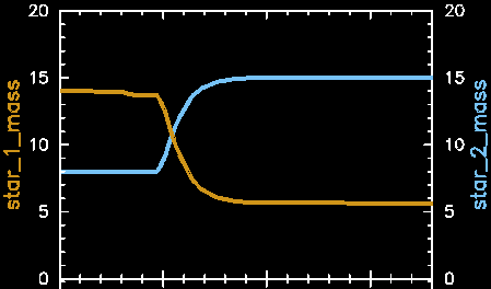
binary is evolving both stars with equal timesteps.
The simulation should end when the donor star (16 M⊙) has started core helium burning and is red and large (R ≈ 340 R⊙). It also has started to develop a convective envelope because it is close to the Hayshi track. The accreting star has become brighter and bloated from the accretion, causing it to also fill its Roche lobe. Because the accretor star fills its Roche lobe, MESA stops.
Whether accretor stars can stably accrete the material they are fed during Hertzsprung gap Roche lobe overflow is uncertain. The later during the Hertzsprung gap the donor fills its Roche lobe, the faster is the flow of material as the thermal timescale of the donor decreases, making it more and more difficult for the accretor star to accrete the material. Here, let’s assume that the two stars in the binary you just created actually will lead to the development of a common envelope and a subsequent merger.
Task 2: Merger Mass Assuming no mass is lost during the merger, what will be the mass of the merger product?
The final masses of the two stars were 15.4 M⊙ and 8.3 M⊙. If there is no mass lost, the merger should contain all of this matter, and thus have a mass of 23.697971 M⊙. (The copious significant digits are unfortunately useful, so hold on to them.)
Constructing a Fake Merger Product
MESA has capabilities to create and evolve many different types of structures, not all necessarily physically motivated. To mimic a merger product, let’s use this capability and fake the resulting star.
To be able to evolve a merger product, we must first create the model to start from. To do this, we begin with making a model with the right mass, and then improving it to also have the composition we want.
Task 3: Faking a Merger
We need to create a starting model that has the total mass of the merger product. To do that, use the work directory 2_relax_mass. Start with studying the inlist_project file.
We need a model to start from, it doesn’t matter very much which one, but we have a model with quite close mass created from the previous step -- the final model for the donor. Start the mass relaxation from this model and also adjust the total mass that you would like to reach. Compile and run the model. See how you reach the appropriate mass in the terminal.
MESA Warning: Use a Precise Mass!
For the best results, set the total mass to the precise sum of the two component star masses, to many significant digits. If you don't, you may run into convergence issues when we change the composition of the merger product. We're not entirely sure why this is, but it likely has to do with how the mesh is set up in the initial mass in that step.
First update the saved model's filename. You could copy the final model for the donor from the previous directory and simply use 'M1.mod', or you can reference it directly from the previous work directory, which might be nice if this directory should be run in succession with the previous. We'll do that here:
! inlist_project
&star_job

  ! Load saved model
    load_saved_model = .true.
    saved_model_name = '../1_evolve_binary/M1.mod'
We also need to update the final mass after relaxation to 23.697971 M⊙:
! inlist_project
&star_job
  ! other parts of star_job namelist omitted

  ! Relax the mass
    relax_initial_mass = .true.
    new_mass = 23.697971
The final mass after running can be confirmed from the terminal output (6th column, first row):
__________________________________________________________________________________________________________________________________________________

       step    lg_Tmax     Teff     lg_LH      lg_Lnuc     Mass       H_rich     H_cntr     N_cntr     Y_surf   eta_cntr   zones  retry
   lg_dt_yr    lg_Tcntr    lg_R     lg_L3a     lg_Lneu     lg_Mdot    He_core    He_cntr    O_cntr     Z_surf   gam_cntr   iters
     age_yr    lg_Dcntr    lg_L     lg_LZ      lg_Lphoto   lg_Dsurf   C_core     C_cntr     Ne_cntr    Z_cntr   v_div_cs       dt_limit
__________________________________________________________________________________________________________________________________________________

       1055   8.209733   3943.130   4.977102   5.120229  23.700000  18.373522   0.000000   0.003426   0.252000  -3.909521   1524      0
  -2.476449   8.209733   2.890977   3.731701   3.810187 -99.000000   5.326478   0.993923   0.000079   0.006000   0.031750      5
 1.3338E+07   2.840863   5.120012   4.500233 -99.000000  -8.671538   0.000000   0.000230   0.001119   0.006077  0.000E+00  max increase
The entropy inside stars typically increases with radius. Entropy can be resembled with the ability to float – higher entropy material floats easier and therefore ends up on the surface. When assembling the two merging stars and deciding what the composition structure of the merger product should be, sorting it according to the specific entropy of the zones is, therefore, a method that has been used when modeling merger products (e.g., Lombardi et al. 2002).
Task 4: Adjusting the Composition
You have now produced a model with the appropriate mass, but the composition is still not updated. To do that, we need to also relax the composition according to a predetermined structure that is provided in a text file. For this exercise, use the work directory 3_relax_composition. Begin with studying the inlist_project file and locate where the relaxation is treated.
- Fill in and set up so that the simulation will start from the model with correct mass.
-
You can see that we need to provide a text file with a composition structure. You have two options here:
-
Create it yourself if you have
pythoninstalled on your computer - then run the python script calledconstruct_merger_composition.pyinside your old work directory1_evolve_binary. OR -
Use pre-created composition files located in the folder
merger_composition_files. For this exercise, you'll want to usemerger_composition_16_8_HG.txt, which corresponds to coalescence as the primary star crosses the Hertzsprung Gap.
-
Create it yourself if you have
- Compile and run the model. See how the composition of the star changes.
Composition Creation Tip: Using construct_merger_composition.py
Do you have python installed (along with numpy) and want to create your own composition profile file? Excellent! The script construct_merger_composition.py should be located at the same level as the other working directories, directly inside maxilab. To use it, do the following (assuming you are in maxilab):
-
Copy the script into
1_evolve_binary:
cp construct_merger_composition.py 1_evolve_binary/ -
Navigate to
1_evolve_binaryand execute the script:
cd 1_evolve_binary
python construct_merger_composition.py -
Copy the resulting file,
merger_composition.txtinto the work directory where we need it,3_relax_composition:
cp merger_composition.txt ../3_relax_composition/ -
Now navigate to the proper working directory:
cd ../3_relax_composition
What's this script doing?
Go ahead an look inside! It loads the two models into numpy arrays, concatenates them together, sorts them by specific entropy, and then writes the new structure out in a format that the composition relaxing routines can understand.
Composition Creation Tip: Using pre-made composition profiles
Don't have python and numpy installed, or don't care to deal with it? That's okay, too. Just copy the profile you want from maxilab/merger_composition_files into 3_relax_composition. You'll need to change the name of the file to simply merger_composition OR adjust the name of the file read in (set in inlist_project) to match the file you copied in.
To load the correct model, we want load the model we produced in 2_relax_mass. Again, we could manually copy that file into 3_relax_composition, or we could provide a path to the model in the original directory. The second option is more robust to running the directories in succession, so we'll show that again.
! inlist_project
&star_job

  ! Load saved model
    load_saved_model = .true.
    saved_model_name = '../2_relax_mass/relaxed_mass.mod'
Now note the following lines that tell star to change the composition of the file:
! inlist_project
  ! Relax the composition of the star
    relax_initial_composition = .true.
    num_steps_to_relax_composition = 250
    relax_composition_filename = 'merger_composition.txt'
MESA star will try to relax the composition of the star so that it matches the configuration specified in a file called merger_composition.txt. Either copy the result of running the construct_merger_compositon.py script into this working directory (see box above) or copy a composition profile from the merger_composition_files directory and rename it to merger_composition.txt (or change the value in the control to match the name of the file; again, see above).
After compiling and running you should see a rather strange abundance profile in the pgstar abundances panel:
Entropy sorting can give rise to an erratic composition structure, which can be seen in the pgstar window. This is a known behavior, but probably not completely physically realistic. However, as you notice during the composition relaxation, the merger product develops a deep convective envelope (look at the Kippenhahn diagram), which quickly will smoothen the strange composition profile in the next step when we evolve the model with time.
Evolving the merger product
Task 5: Evolve the Merger Product
Now your model is ready to be evolved with time, so pick the resulting model from your composition relaxation, merger_start.mod, and place it inside the directory 4_evolve_merger. Import the model as a starting model. Set the model to stop when the central helium mass fraction reaches 0.5. Compile and run your model.
From within 3_relax_composition, copy the final model to the next directory:
cp merger_start.mod ../4_evolve_merger/
and then navigate to that directory:
cd ../4_evolve_merger
To load that model, add/update the usual controls in the star_job namelist in inlist_project:
! inlist_project
  ! Load saved model
    load_saved_model = .true.
    saved_model_name = 'merger_start.mod'
(Or we could directly link to the previous directory by pointing to ../3_relax_composition/merger_start.mod). The stopping condition is then (in the controls namelist)
! inlist_project
   ! Stopping condition: central he4 mass fraction
     xa_central_lower_limit_species(1) = 'he4'
     xa_central_lower_limit(1) = 0.5
And as usual, compile and run with ./mk && ./rn
Task 6: Analyze the Merger Product Answer the following questions about the merger product evolution:
- What happened to the merger product?
- What regions of the star are convective?
- What is the effective temperature? What is the radius? What is its surface gravity?
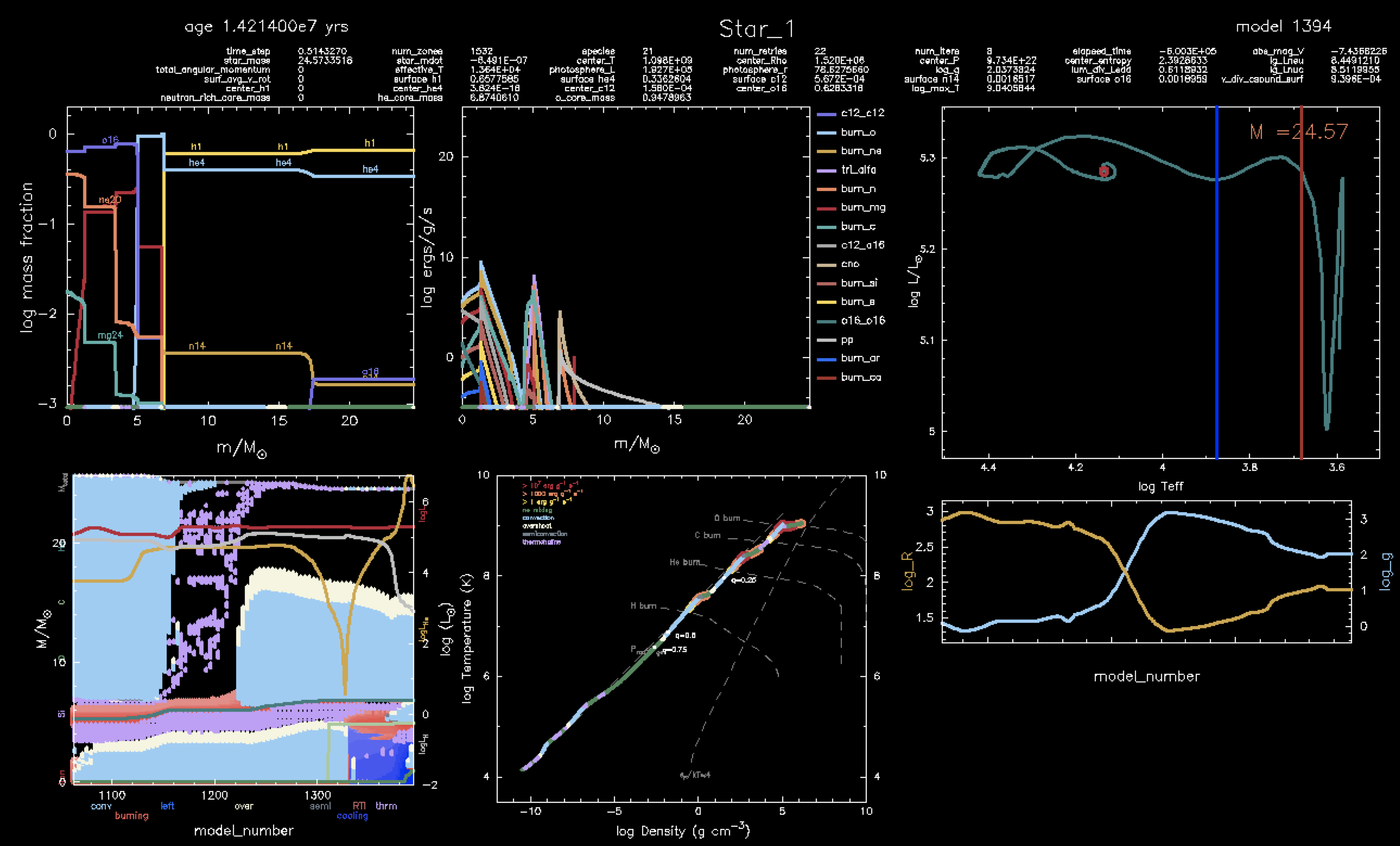
- Do you think the merger product could be confused with a single main sequence star?
Let's take a look at one of the final frames from the pgstar dashboard
- What happened to the merger product? The star contracted and heated up. The composition profile has smoothened.
- What regions of the star are convective? During central helium burning, the helium-burning core is convective as well as the hydrogen-burning shell. The convective layer covering the hydrogen-burning shell extends over ≈ 8 M⊙ and therefore reaches into the non-burning envelope as well.
- What is the effective temperature? What is the radius? What is its surface gravity? The final effective temperature is approximately 24,000 K, the radius is about 23 R⊙, and the surface gravity is about log g ≈ 3.
- Do you think the merger product could be confused with a single main sequence star? Apart from the surface gravity being somewhat low for main sequence stars, the effective temperature and radius match well with the expectations for main sequence stars. The luminosity is also similar. This star could most likely be confused with a single main sequence star.
The contraction of merger products is thought to result from the mass gain: suddenly the helium core constitutes a much lower fraction of the total stellar mass compared to before. A thick convective layer has also been discovered in stellar evolutionary models that burn helium as blue supergiants (e.g., Klencki et al. 2020). These characteristics of the interior structures of merger products differ from what is expected for single stars with the same temperatures and luminosities.
Bonus Task 7: How to Recognize It? The helium-core burning stage is the second longest evolutionary stage of a star, after the main sequence when the star burns hydrogen in the center. Assuming merger products contract like yours, can you think of ways to distinguish them from regular, single, main-sequence stars?
On the surface, the merger products seem similar to main sequence stars, possibly with a little low surface gravity. With data from large spectroscopic surveys it may be possible to identify a subgroup of hot stars with lower surface gravity. However, this could be hard. Asteroseismology could provide the best constraints, since with pulsations it could be possible to characterize the core size and possible convective layers.
Final Evolutionary Stages
The merger product is massive enough to eventually undergo core collapse. How does this supernova progenitor look like? Here are some rough characteristic effective temperatures for massive stars (adopted from Drout et al. 2009):
- Blue Supergiant (BSG): > 7,500 K
- Yellow Supergiant (YSG): 4,800 K – 7,500 K
- Red Supergiant (RSG): < 4,800 K
Task 8: Evolve towards death Change the stopping condition in your model to central carbon depletion and restart your merger product. What happens to the star? According to the giant star definitions above, what type of star do you think it is at death?
To change the stopping condition, we update the stopping condition from Task 5 to the following:
! inlist_project
   ! Stopping condition: central he4 mass fraction
     xa_central_lower_limit_species(1) = 'c12'
     xa_central_lower_limit(1) = 1d-3  ! or something else sufficiently small
And then we restart rather than start fresh with ./re.
To analyze the evolution and final fate of the merger product, let's look at the final fram of the pgstar dashboard:
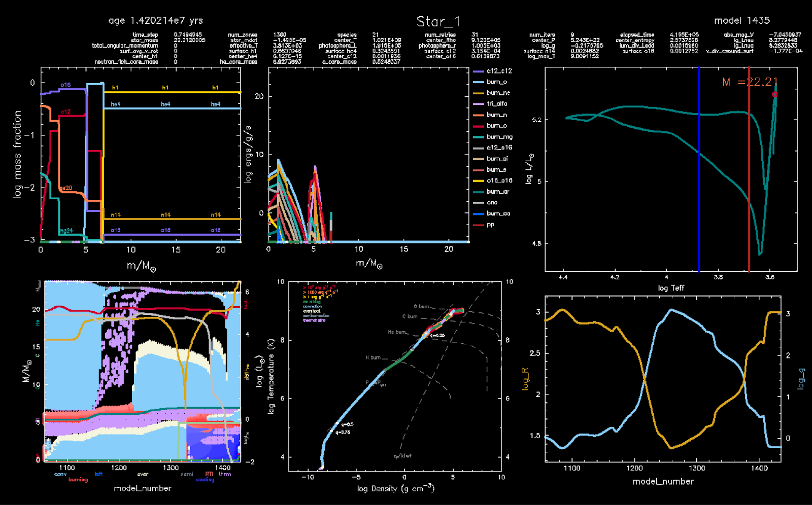
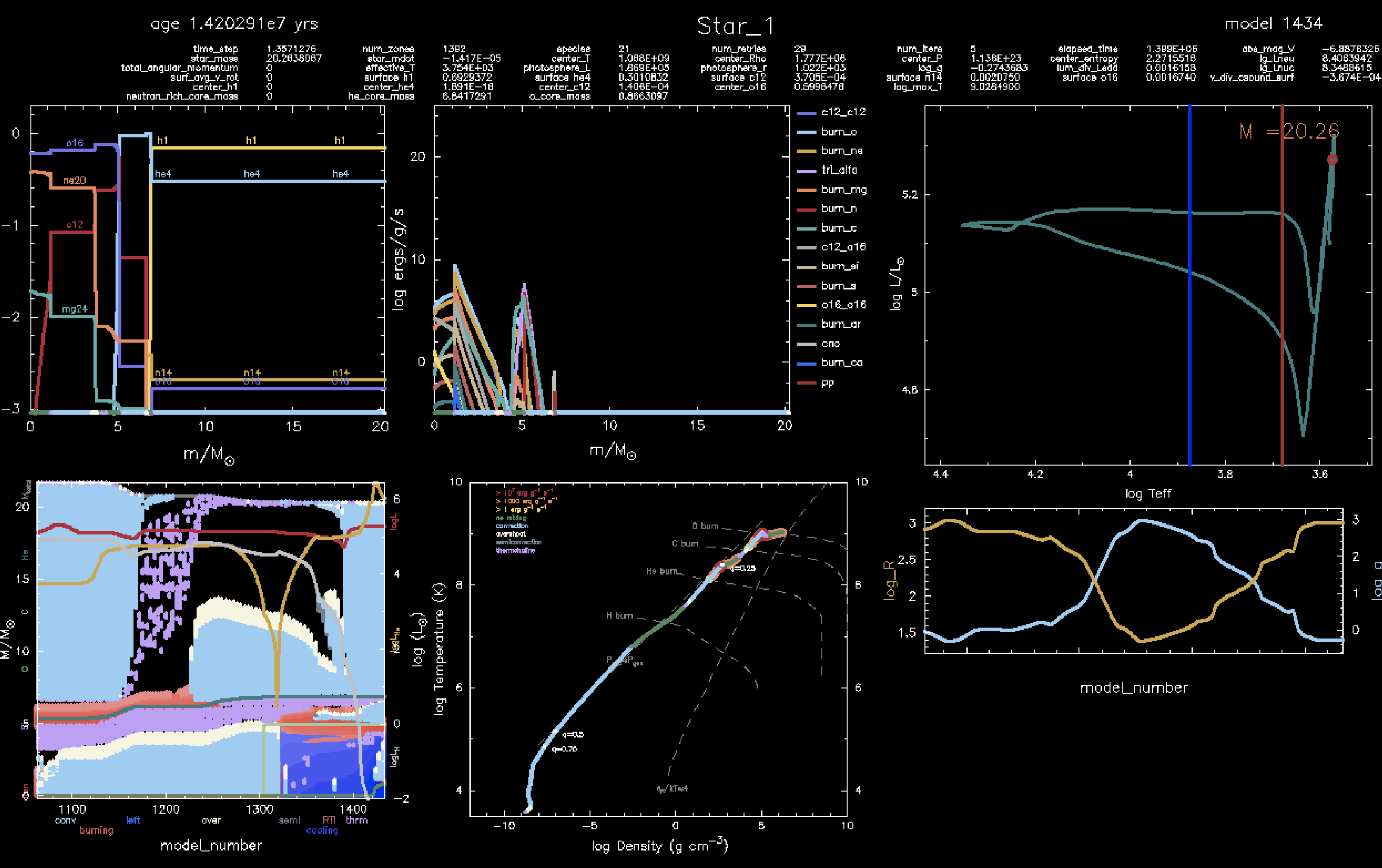
The star expands and cools again, reaching ~ 1,000R⊙ and 3,800 K. The star develops again a deep convective envelope. At death, this merger product should be a RSG. Maybe there is extra ejecta mass?
Blue Supergiants as Merger Products – from Life to Death
Do all merger products behave like the model you just created? This could mean that regular single stellar population synthesis models under-predict the number of BSGs, since massive single stars are thought to burn helium as RSGs, while your merger product burns helium as a BSG. Merger products have even been suggested as responsible for the blue supergiant progenitors of some supernovae, like SN 1987A (e.g., Podsiadlowski et al., 1990, Menon et al., 2017). Let’s explore how common these blue supergiant phases may be and whether they can last to the end stages of stellar life.
Task 9: Change Component Masses Make a new merger product with different masses: each person at a table chooses a new combination of masses among the following options:
- 18 M⊙ and 10 M⊙
- 18 M⊙ and 9 M⊙
- 16 M⊙ and 10 M⊙
- 16 M⊙ and 6 M⊙
- 11 M⊙ and 8 M⊙
Follow the same steps as previously to create a new merger model. For the models to run smoothly, make sure to use the masses from the terminal output when calculating the total mass of the merger product. If you use the pre-computed composition profiles, make sure to pick the one corresponding to your initial component masses.
What is the stellar type of your merger product
- during helium core burning?
- at death (carbon depletion)?
Once you have identified the primary and secondary masses, assemble the ZAMS models you need from the ZAMS_models directory. Then follow the steps from tasks 1, 3, 4, 5, and 8, being careful to update any models and/or composition files that you need to copy from directory to directory.
When you are ready to identify the SN progenitor type, stop the merger product evolution when the central helium abundance is at 0.5 and look at its position on the HR diagram (the left of the blue line is a blue supergiant, to the right of the red line is a red supergiant, and between is a yellow supergiant), or read off the effective temperature and look at the definition given above. Then adjust the stopping condition to central carbon depletion and restart, checking the final progenitor type again.
You should find the following progenitor types (including the first merger model we did earlier):
| M1 | M2 | Core He Burning | Carbon Depletion |
|---|---|---|---|
| 16 M⊙ | 8 M⊙ | Blue Supergiant | Red Supergiant |
| 18 M⊙ | 10 M⊙ | Blue Supergiant | Blue Supergiant |
| 18 M⊙ | 9 M⊙ | Blue Supergiant | Red Supergiant |
| 16 M⊙ | 10 M⊙ | Blue Supergiant | Blue Supergiant |
| 16 M⊙ | 6 M⊙ | Blue Supergiant | Red Supergiant |
| 11 M⊙ | 8 M⊙ | Blue Supergiant | Blue Supergiant |
As you can see, all are blue supergiants during Core He Burning, but the final state is more varied. Let's take a look at a couple final snapshots to see where these classifications come from. First is the result of merging a 16 M⊙ star with a 10 M⊙ star:
And now for the merger of a 16 M⊙ and a 6 M⊙ star:
Why the Difference?
The convective envelopes in the two models are quite different. For the BSG, the conevective envelope does not reach out to the surface, while in the RSG, the convective envelope does indeed reach the surface. This is likely related to the different final radii, and thus final effective temperatures.
However, the direction of this causality is not well understood. Does the smaller radius cause the smaller convective envelope in the BSG, or the other way around?
Another thing to note is the mass ratios of the two initial stars. More equal mass ratios tend to create BSGs, while more extreme mass ratios tend to create RSGs. This may manifest in different core-envelope mass ratios in the merger, which may lead to the bifurcation in SN progenitor types.
Coalescence at Different Evolutionary Stages
Binary stars can merge, for example, because of too long or too short an orbital period, or because of extreme mass ratio. We have explored scenarios when the merger occurs because the binary has a very wide orbit - now let's look at how the merger product evolves if the stars merged already during the main sequence evolution.
Task 10: Evolve a Main Sequence Merger
Start from your first merger model (with 16 M⊙ and 8⊙ stars), but change the initial period to 1.5 days and follow the same steps (tasks 1–5). There is a pre-computed composition file for this main sequence merger in the folder merger_composition_files called merger_composition_16_8_MS.txt, but you can also compute your own with the python script.
Does the merger product still burn helium as a blue supergiant? Does the evolution in the HR diagram remind you of something?
Note: this model takes a minute to find a good starting point, but it will get going.
With this short initial orbital period, the stars coalesce when they are both burning hydrogen in their cores. Thus, the resulting merger product also starts with a hydrogen-burning core. Check out the last pgstar frames from the initial binary evolution below.
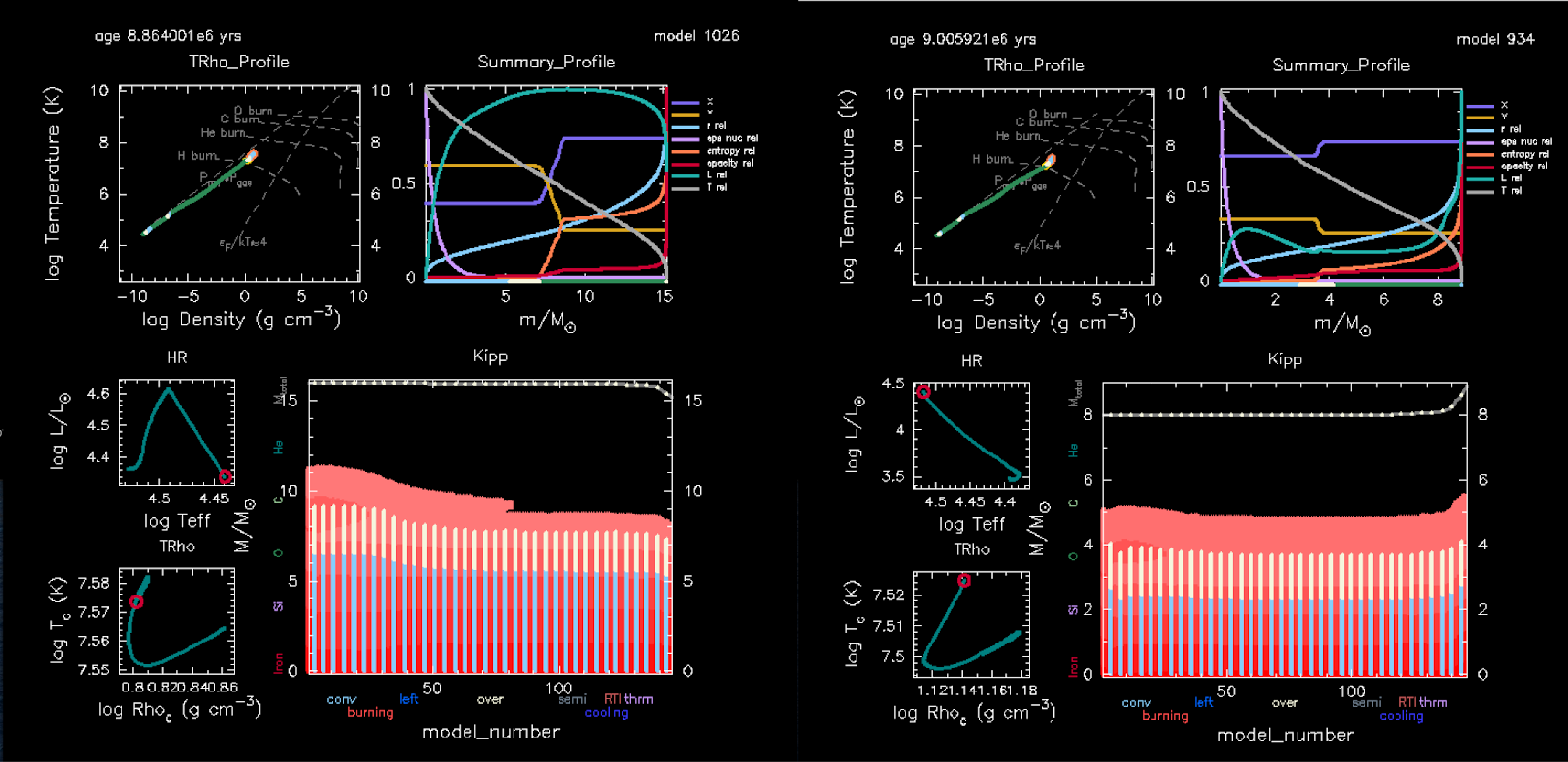
After rescaling the mass and relaxing the composition, the resulting merger product is also just fusing hydrogen in its core rather than helium. For an example, see the frame below captured during the relaxation process:
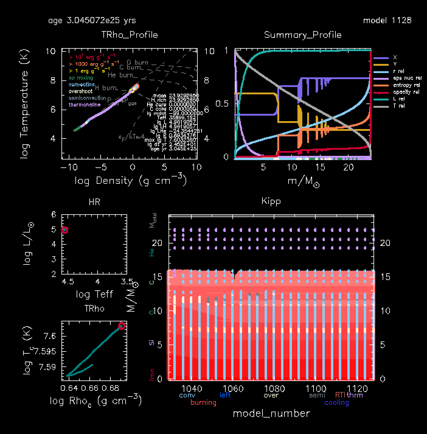
After the merger product exhausts its core hydrogen supply, subsequent helium burning is slow in MESA due to a prodigious wind mass loss rate. However, through this phase of burning, the HR diagram already shows us the interesting result: the evolution is similar to a single massive star. It starts off as a hydrogen-burning giant, and then upon depletion, crosses the hertzsprung gap and becomes a red supergiant during core helium burning.
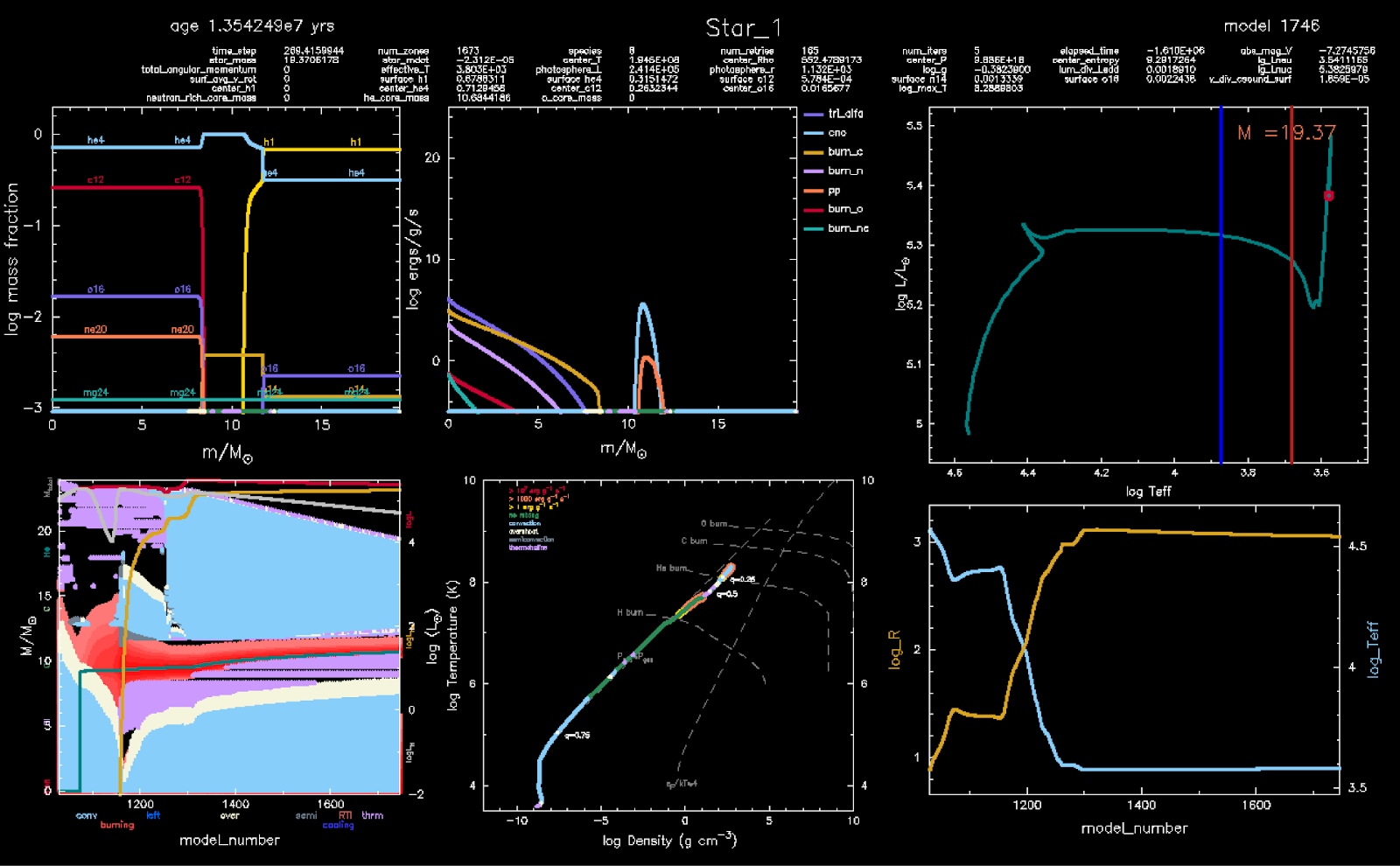
BONUS: Rotation of Merger Products
After the coalescence of two stars, some angular momentum is thought to remain, causing the merger product to spin. Let's invoke rotation in the merger product before evolving it further.
Bonus Task 11: Invoke Rotation
We'll modify the most recent merger product (the main sequence merger) to add rotation to the merger product and study how it evolves. So we'll only be working in 4_evolve_merger.
-
To make sure that the model we invoke rotation in has fully adjusted, start with evolving
merger_start.modfor 10 model numbers and save a model at the end of the run. -
Look through
star_job.defaultsfor how to make the star rotate. Change the rotation flag to a new rotation flag. Set the spin rate (in Ω/Ωcrit) to 0.5. Assume 60 steps of relaxation for the model to reach the right spin rate. -
Activate a panel showing rotation in the pgstar window. Find it by searching for
ROTATION. - Start a new run from your saved model.
To save the non-rotating, but adjusted model, we need to set a stopping condition that makes it stop after 10 timesteps. It's easiest to do this by zeroing out the model number and setting a stopping condition of a maximum model number of 10. Note that all of this is happening in 4_evolve_merger, using a model that has already had its mass and composition relaxed.
in star_job:
  ! inlist_project
  ! zero out model number
    set_initial_model_number = .true.
    initial_model_number = .true.
and in controls:
  ! inlist_project
  ! stop after 10 timesteps
    max_model_number = 10
We also need to save a model at the end of this run. You can call it anything, but we'll assume you called it rot_prep.mod. In star_job:
  ! inlist_project
  ! save model in preparation of turning on rotation
    save_model_when_terminate = .true.
    save_model_filename = 'rot_prep.mod'
We'll want to run this model (./rn) to save the adjusted model. We'll then load that model in the next step. So now we'll adjust the name of the loaded and saved models, as well as adding the necessary rotation controls, all in star_job:
  ! inlist_project
  ! Load saved model
    load_saved_model = .true.
    saved_model_name = 'rot_prep.mod'

  ! save model in preparation of turning on rotation
    save_model_when_terminate = .true.
    save_model_filename = 'end.mod'

  ! Invoke rotation
    ! first turn rotation on
    change_rotation_flag = .true.
    new_rotation_flag = .true.

    ! now set rotation in rate in terms of the critical rotation rate
    set_omega_div_omega_crit = .true.
    new_omega_div_omega_crit = 0.5

    ! allow adjustment to rotation rate to happen over many timesteps
    relax_omega_div_omega_crit = .true.
    num_steps_to_relax_rotation = 60
A rotation panel is already provided in inlist_pgstar; you only need to replace an empty string with the commented string next to it:
  ! inlist_pgstar
  ! ! ! ! ! DISPLAY ROTATION  ! ! ! ! ! !
  ! The second panel
  History_Panels1_yaxis_name(2) = 'surf_avg_v_rot'
  History_Panels1_other_yaxis_name(2) = ''
  ! ! ! ! ! ! ! ! ! ! ! ! ! ! ! ! ! ! ! !
And then you are ready to run this new model that loads the adjusted one with ./rn.
Bonus Task 12: Spindown What was the initial equatorial rotation rate of the merger product? What is it at the end of the central hydrogen burning phase?
To estimate the desired velocities, take a look at the final frame of the pgstar dashboard, shown below.
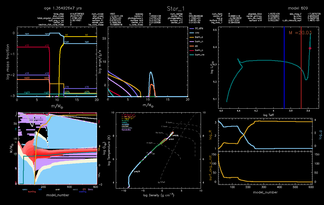
Look at the history panels in the lower right. The lower one is the new panel we just added, and it shows that the initial equatorial rotation rate is approximately 150 km/s, while at TAMS (around model 40, when radius finishes its initial expansion), it has spun down to around 25 km/s.