This guide is meant to supplement the live tutorial given by Andrew Cumming and Bill Wolf at the
Bursting the Bubble
workshop hosted at
the Lorentz Center
at the
Leiden University
in June 2019. Here, we'll help new users of Modules for Experiments in Stellar Astrophysics (MESA) get started with the tool to model thermonuclear bursts on white dwarfs and neutron stars. We'll leave this tutorial online for at least awhile afterwards in the hopes that it proves to be a helpful guide for getting started with bursts in MESA, but these instructions are aimed at participants going through the tutorial at the workshop. It will likely fall out of date as the interface of MESA changes in its development and the hyperlinks on this page become outdated.
You should complete Part 0 before the tutorial begins on Tuesday afternoon. If you have issues, reach out to Andrew on Monday to get set up in advance of the tutorial. You should use the following versions of MESA and the SDK:
MESA Version
11701
SDK Version
20190503 (Mac or Linux)
Throughout this page, monospaced text on a black background, like this: echo "Hello, World!" represent commands you can type into your terminal and execute, while red monospaced text like this: mass_change = 1d-9 represent file names or values that you might type into a file, but not something to be executed.
Part 0: Before You Arrive
Installing MESA and its prerequisites is not particularly difficult for most users and systems, but it can take a little time to download and compile, so you should do this before the tutorial, and ideally early enough so that you can ask Andrew for help on Monday.
Installing the SDK
While MESA can be run on custom compilers and other tools with a fair amount of work, the MESA SDK is the easiest way to get started. Get the SDK with the link below, and follow the instructions for your particular system, noting the prerequsites.
Your first step is to install the SDK and confirm that it works on your system by trying which gfortran in a terminal to confirm that the SDK version of gfortran is being used.
Warning for macOS Mojave Users
On macOS 10.14 (Mojave; and perhaps later versions, too), you may also need to install the development header files. These ship as a standard part of Mojave, but must be installed by hand. To do so, run the command
open /Library/Developer/CommandLineTools/Packages/macOS_SDK_headers_for_macOS_10.14.pkg
This step may need to be repeated whenever you upgrade to a new release of the Xcode command-line tools.
Installing MESA
Once the SDK is properly installed, it's time to install MESA on your machine. This amounts to downloading a zip file, moving it to where you want, and executing an install script.
With MESA and its SDK installed, it's time to do a first run to make sure eveything is working properly. Follow the official tutorial and feel free to play around a bit once you've gotten the hang of it!
In that simple exercise, you learned how to create a new simulation in MESA. You then went into this new work directory, compiled it, and ran it. We now summarize these steps, as they are the most common path to creating a new simulation:
Make new work directory: cp -r $MESA_DIR/star/work tutorial
Enter that directory: cd tutorial
Compile the work directory: ./mk
Start the simulation: ./rn
MESA Best Practice: Work Directories
Never run simulations from within your local installation of MESA. Depending on the value of $MESA_DIR is, you may not actually be compiling against the installation you think you are, and in general it's best to not mess with the source code.
Instead, always make a copy of the standard work directory $MESA_DIR/star/work or start from one of the test cases in $MESA_DIR/star/test_suite (though those require a bit of work to be truly customized).
You also should have learned a little about the inlist files that control the simulation as well as how to start a simulation (./rn) and restart from a photo (./re photo, where photo is one of the files in the photos directory). Confirm that you know how to do all these things, and that you saw the terminal output and real-time plots indicated in the "getting started" tutorial as you ran the simulation before moving on.
If you're looking for a more in-depth tutorial into general use of MESA that will really prepare you for our work with bursts, Josiah Schwab has prepared a great introduction to using inlists and much more for the MESA summer school.
MESA is a modular code, so different parts of the code handle different tasks needed in modeling stars. Most often, you'll be using the star module, which uses the other modules to compute a stellar model and evolve it in time. Let's take a look at the structure of a typical work directory.
Structure of a Work Directory
Your tutorial work directory had the following files and directories. Click on each to learn about what each file or directory does.
Instructions for how to model the star, including models to load, timestep controls, microphysics options, and on-screen plots. Often this punts to other inlist files to separate different functionalities.
MESA Output
Output from a MESA simulation is stored in the LOGS directory (though you can change the name of this directory in the inlist). There are two primary types of output files: histories and profiles. Each simulation has one history file, typically called history.data, that records how scalar quantites related to the model like age and luminosity change through time. There can be many profiles saved, and each file gives a snapshot of quantities that vary throughout the entire star, like density and temperature. There is one other file, called profiles.index. This file relates the names of profiles to their corresponding model number (timestep) in the history file.
How often profiles are written to disk, how many there are allowed to be before they start to get overwritten (they can get quite large!), how often a line is recorded in the history file, how the files are named, and many other output details can be customized in the inlist. The exact types of data that are recorded in the history and profiles are controlled in two other files that may or may not be in your work directory: history_columns.list and profile_columns.list. If these files do not exist in your work directory, they are read from their default location in $MESA_DIR/star/defaults.
To enable/disable different columns in the output files, open the corresponding columns file and uncomment the names of columns you want to output, and comment out those that you don't.
MESA Best Practice: Output Column Files
Don't edit the default columns files so that you don't get unexpected behavior in other projects. Instead, copy them into your local work directory via
Then, edit these files in your local work directory. MESA will always look for these files in the local directory before falling back to their default versions.
You can see a summary of each of the important files for MESA output by clicking on each of them below
Data file with one line for each model number/timestep (or every n models. The columns used are determined by the uncommented lines in history_columns.list. You can set the frequency for outputting a line with the history_interval control in the controls namelist.
The main MESA website has suggestions for how to work with MESA output, including a recommended python library for reading and plotting it after the simulation is over.
When you execute ./rn or ./re photo in a vanilla work directory, MESA reads instructions from inlist. The name of the file must be "inlist". The inlist is composed of three namelists, which are series of name-value pairs, set off at the top by &namelist where namelist is the name of the namelist, and concluded by a line with a single slash: /. See for example, the contents of inlist from the initial tutorial.
Contents of inlist
! this is the master inlist that MESA reads when it starts.! This file tells MESA to go look elsewhere for its configuration! info. This makes changing between different inlists easier, by! allowing you to easily change the name of the file that gets read.&star_jobread_extra_star_job_inlist1=.true.extra_star_job_inlist1_name='inlist_project'/! end of star_job namelist&controlsread_extra_controls_inlist1=.true.extra_controls_inlist1_name='inlist_project'/! end of controls namelist&pgstarread_extra_pgstar_inlist1=.true.extra_pgstar_inlist1_name='inlist_pgstar'/! end of pgstar namelist
In MESA star, there are three types of namelists, and all three are in this example inlist. Click through each namelist below to learn what each is used for. You can also find documentation for each namelist on the MESA home page that is automatically generated from the defaults files.
Contains controls for the program that evolves the star. For instance, whether or not the program should load a model or save one. Also tells the program where to find opacity and eos tables, what nuclear network to use, and other fundamental options. Defaults are found in $MESA_DIR/star/defaults/star_job.defaults.
In this case, each namelist only has two controls set. The first tells the namelist to read values from another file, which must also be set up in this way. The second tells it the name of the file to read in.
MESA Best Practice: Multiple Inlists
It may seem needlessly complicated to have inlists pointing to each other instead of putting all controls in one inlist, but this is often very convenient, since large inlists can become cumbersome.
A common convention is to have a "favorites" list in an inlist, named something like inlist_common. Here you have your preferred default settings. Then in another inlist, you put the truly unique quantities that differentiate this simulation from others.
pgstar namelists can also become quite lengthy, so it is extremely common to see them broke out into their own file, typically called inlist_pgstar.
There's nothing stopping you from just having one giant inlist with all of your controls, though!
For completeness, let's look at the contents of inlist_project to see some more typical namelists.
Contents of inlist_project
! inlist to evolve a 15 solar mass star! For the sake of future readers of this file (yourself included),! ONLY include the controls you are actually using. DO NOT include! all of the other controls that simply have their default values.&star_job! begin with a pre-main sequence modelcreate_pre_main_sequence_model=.true.! save a model at the end of the runsave_model_when_terminate=.false.save_model_filename='15M_at_TAMS.mod'! display on-screen plotspgstar_flag=.true./!end of star_job namelist&controls! starting specificationsinitial_mass=15! in Msun units! options for energy conservation (see MESA V, Section 3)use_dedt_form_of_energy_eqn=.true.use_gold_tolerances=.true.! stop when the star nears ZAMS (Lnuc/L > 0.99)Lnuc_div_L_zams_limit=0.99d0stop_near_zams=.true.! stop when the center mass fraction of h1 drops below this limitxa_central_lower_limit_species(1)='h1'xa_central_lower_limit(1)=1d-3/! end of controls namelist
Note here that there are only two namelists (pgstar is relegated to inlist_pgstar). If you are unfamiliar with fortran syntax, note also the literals for booleans, .true. and .false. as well as how array assignment works, as in xa_central_lower_limit(1) = 1d-3
Warning: Inlist Pitfalls
The syntax of inlists is somewhat strict. While whitespace doesn't matter, please observe the following rules to avoid sadness.
Don't use any mathematical operators in values, only literals (strings, floats, integers, and logicals).
Don't use control statements like if or while
Put controls in their correct namelists. Capitalizaition is not important, but spelling is.
Always use double precision numbers for floats, as in 1d3 rather than 1000.0 or 1e3 (technically not mandatory, but this will give more consistent and reproducible results)
Some of these shortcomings can be mitigated by using a third-party tool, MesaScript, but this is beyond the scope of this tutorial.
Compiling, Running, and Restarting
So you have set up a new work directory, edited your inlists with controls found in $MESA_DIR/star/defaults, and you're ready to run your model. First, you need to compile!
Compiling and Troubleshooting
To compile your code, execute ./mk. You should see a few lines fly by on your terminal, and hopefully no errors. If you do have errors, check the following:
Make sure you have $MESASDK_ROOT set up via echo $MESASDK_ROOT
Make sure the SDK is initialized. A quick indication that this is fine is to run which gfortran and making sure the resulting path points to the gfortran in the SDK.
If you've made edits to src/run_star_extras.f (more on this later), check the error output for indications that you have bugs in your code.
Try first running ./clean and then do ./mk
Finally, something may be wrong with your MESA installation, so try recompiling it with
cd $MESA_DIR./clean./install
And if none of that works, try completely re-installing MESA
Running and Real-time Output
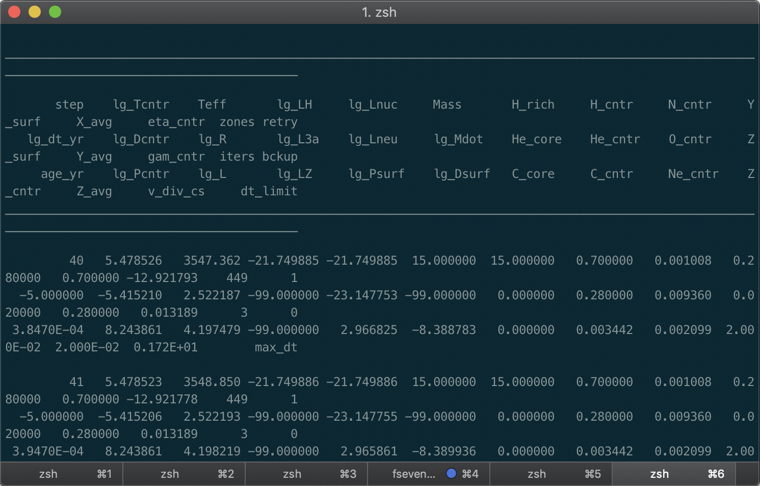
Assuming that you have successfully compiled your work directory, start the simulation with ./rn. Soon, terminal output should indicate that models are being computed. Note that you will want your terminal to be wide enough to fit each step's data without wrapping. Your terminal should be at least 146 columns wide for proper viewing.
Terminal output when the terminal is too small. The lines wrap and it becomes very difficult to interpret.
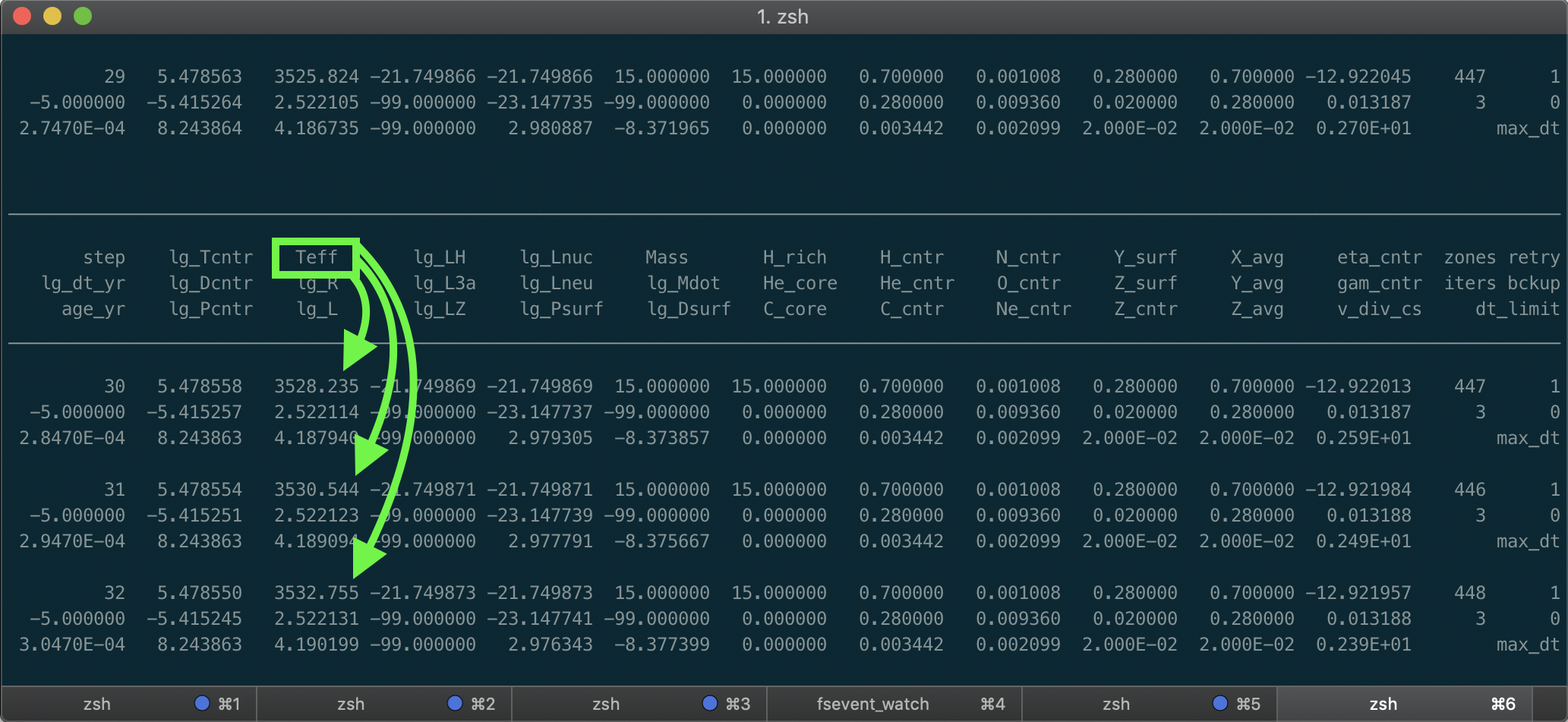
Terminal output when the terminal is wide enough. Each chunk of three lines give summary data for each timestep. The headers are printed every few printed timesteps and guide you to the meaning of each number. In this figure, we indicated that the first row of the third column always gives the effective temperature in our stellar model.
These data can be helpful, but usually real-time plots from pgstar are a better way to understand how your stellar model is evolving. In order to see these plots, you'll need to properly configure your pgstar namelist (not covered here) and set pgstar_flag = .true. in your star_job namelist. If you have this set up, as in the standard work directory, plots (in this case a temperature-density profile as well as an HR diagram track) will appear in their own windows as the terminal output begins.
Restarting and Photos
Sometimes you'll have to stop your simulation to adjust the inlist or because you need the computing power for some other task. You can do this by executing ctrl-C. But now do you have to restart the whole simulation? Fortunately, no! You can restart from a "photo". A photo is a snapshot of your stellar model dumped into a binary file.
By default MESA saves a photo to the photos directory every 50 timesteps. They are named such that the last three digits are the same as the last three digits of their corresponding timestep. To save disk space, they are overwritten every thousand timesteps. That is, step 1050 will be saved as the file x050 in photos (where the x is literally there), and it will be overwritten when step 2050 does the same thing. To give longer-term access, every thousand timesteps will remain indefinitely, so timesteps 1000 and 2000 will save photos 1000 and 2000, respectively.
To restart from photo x050, simply execute ./re x050, assuming it exists in photos. inlist will be read again, so you can change commands on the fly, though in practice this is difficult to reproduce, so you should only use this workflow when you are prototyping a simulation.
Warning: Photo Pitfalls
Photos are not the same as saved models.
Photos are...
Binary (not readable by anything other than MESA)
Sensitive to changes in the MESA source, so they will not work reliably on other versions of MESA
A complete record of the star; it is the same as if the simulation had never been stopped
Saved models are...
Plain text and human-readable
Robust to changes in the MESA source, and may be used on different revisions
A mostly complete record, but you may notice small differences between a model that is restarted from a photo compared to one loaded from a model saved at the same timestep with the same inlist.
There's much more to learn about how to bend MESA to your will, including adding your own physics through code, but you know enough now to be dangerous. We'll touch on some more advanced techniques later.
Part 2: Type I X-ray Bursts
In this section we'll get our hands dirty by running a MESA simulation of a Type I X-ray burst. We'll start from a provided inlist and model, and then we'll edit that inlist to reproduce different burning regimes of accreting neutron stars, and finally we'll edit the microphysics used to calculate opacities in the extreme regimes present in neutron stars.
You can find the original slides used for the tutorial here, but the entire exercise is doable on this site alone, and some of the naming conventions have been updated here.
Disclaimer:
The simulations you are going to do here in this part (and the next) are not resolved, use nuclear networks that are too small, and contain other shortcomings that make them quick to run, but not suitable for publication.
A First X-ray Burst
First, create a new MESA work directory somewhere in your local filesystem:
cp -r $MESA_DIR/star/work burst
and have a look inside. You should see the files described above. We will be replacing both inlist_project and inlist_pgstar to instead model an accreting netutron star and to display more pertinent on-screen plots than the defaults in the standard work directory's copy of inlist_pgstar. Additionally, we'll be adding in our own custom history_columns.list (review what that does here) to enable these plots, and a starting model, ns_1.4M.mod, which gives us just the outer regions of a neutron star above an iron substrate (the inner boundary condition is set to a fixed mass, radius, and luminosity).
After downloading the file, unpack it inside the work directory:
tar -zxvf burst.tgz
This should create the four files mentioned above:
inlist_project
inlist_pgstar
history_columns.list
ns_1.4.mod
You may be prompted to overwrite the two inlists. Go ahead and do that. Our custom history_columns.list will specifically allow us to track and plot the following contents:
star_age_hr: this is the model's age in hours (the default star_age is in years, which is too long for our model)
max_eps_he_lgT: the log of the temperature at the location of peak helium burning
log_total_mass he4: the log of the total mass of helium in the model (in M⊙)
Now you should compile and run the model:
./mk ./rn
After some initial terminal output, you should see a pgstar (the plotting side of MESA) window popping up with multiple panels. The entire pgstar output, when strung into a movie, can be seen below.
The upper left panel shows a density-temperature profile of the star, with the surface being on the lower-left (low temperature and density) and the inner-most part of the model in the upper right (high temperature and density). Note how regions of strong burning are indicated with background colors. In the lower left, we have the log of the surface luminosity (gold, left vertical axis) and the number of zones in the model (blue, right vertical axis) plotted as a function of time. Notice how the number of zones automatically increases during the first few bursts to better resolve the burning region. The upper right panel shows the elemental composition as a function of column depth, and the lower right panel shows how the temperature in the helium burning layer varies with the total mass of helium.
You'll see that this last plot spirals in on a fixed point, coincident with the luminosity plot coming to a constant value after a few initial bursts. Evidently, we have found a stable burning solution, where the rate that helium is burned is nearly balanced by the rate it is accreted.
If you let the simulation go to completion, it will stop after 3000 steps. What determines this? Try to figure out what controls this and other physical parameters in this simulation by studying inlist_project.
Challenge: Open inlist_project and identify the following pieces of information.
The stopping condition(s): there could be multiple, but at least one is after computing 3000 models; what line controls this?
The nuclear network in use
The accretion rate
You can learn more about available options in $MESA_DIR/star/defaults/star_job.defaults and $MESA_DIR/star/defaults/star_job.defaults or their online equivalanets for star_job and controls.
There is only one stopping condition, which we already identified as a maximum model number of 3000. The line that sets it is in the controls namelist:
max_model_number=3000
The nuclear reaction network is set in the star_job namelist by these lines:
The first line tells MESA that we want to change from the network in the starting model (even if we are "changing" to the same network), and the second line specifies what network to use. Premade networks can be found in $MESA_DIR/data/net_data/nets.
The accretion rate of this model is 3 × 10⁻⁸ M⊙/yr, as set by the following line:
mass_change=3e-8! rate of accretion (Msun/year)
You are encouraged to further explore what some of the other commands in this inlist are doing.
Burning Regimes
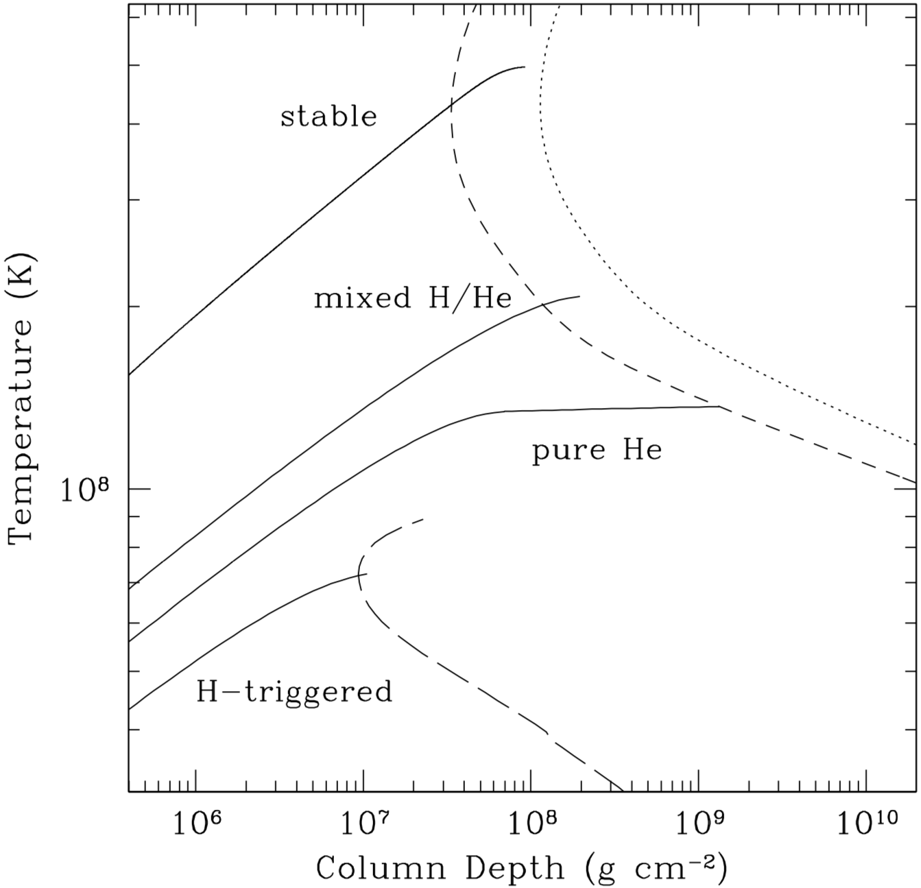
It appears that accreting solar composition material at 3 × 10⁻⁸ M⊙/yr results in stable burning (though incomplete hydrogen burning implies that we don't have a large enough nuclear network). Cumming (2004) reviewed these burning regimes and found the following rough boundaries.
Approximate burning regimes for accreting neutron stars. Note that Keek & Heger (2016) find a new stable burning regime involving stable helium burning to carbon in a narrow range of accretion rates between the pure He and mixed H/He regimes. For simplicity, we neglect that here..
Label
Description
Typical Ṁ
Stable
Both H and He burning are thermally stable
10-8 M⊙/yr
Mixed H/He
Stable H burning (hot CNO cycle) but unstable He burning. He ignites in a H-rich environment (-> rp process)
10-9 M⊙/yr
Pure He
Stable H burning depletes all H before He ignites
10-10 M⊙/yr
H-triggered
Unstable H burning
10-11 M⊙/yr
Profiles of accreting neutron stars in the different burning regimes as described by Cumming (2004)
Our goal is to try to reproduce these burning regime with our simple accreting neutron star model.
Challenge: Edit inlist_project to change the accretion rate, save, and rerun your model (no need to compile unless you change an actual fortran file). Determine what burning regime you are in.
You may want to look at the last burst in your calculation in isolation. We provide a python script to do this, but it assumes you have numpy and matplotlib properly configured on your machine (should be the default with any reasonable scientific distribution of python like anaconda). To use it, download it, move it to your working directory, and execute python plot_lc.py after your run is over. Does your burst look like a Type I X-ray burst?
To change your Ṁ, you need to adjust the following line:
mass_change=3d-8
Specifically, change 3d-8 to a different value, like 1d-8 to set Ṁ=10-8 M⊙/yr.
Below are videos of four models run at the "typical Ṁ's" from the table above.
Ṁ=10-8 M⊙/yr. Similar to our first burst, this goes through a few bursts that weaken until we reach a stable configuration.
Ṁ=10-9 M⊙/yr. We get multiple bursts that seem to fall into a pattern, but then ease into a different regime where helium burns more slowly to Carbon. We'll put this in the "Mixed H/He" range, as Hydrogen appears to burn steadily while He is going through bursts.
Ṁ=10-10 M⊙/yr. Hydrogen burns steadily as a helium layer builds up. We don't actually get to the helium flash, but it is inevitable, so we are in the "Pure He" range.
Ṁ=10-11 M⊙/yr. Now even Hydrogen burns unstably, as the layer builds up and burns away in a cyclic fashion. No He flash occurs in this video, but it would eventually happen after a large number of Hydrogen bursts.
Missing Physics
As we said in the disclaimer, these models are all missing some important physics. Here are just a few:
Mixed H/He Bursts
We need a large network to follow the rp-process. The small network we are using in our model limits the amount of hydrogen burning, so that there is a lot of leftover hydrogen and the bursts have low peak luminosities.
Helium Flashes
These flashes reach Eddington luminosity. We need to be able to follow the expansion and wind. You will find that the code has trouble for low hydrogen fractions when the luminosity approaches Eddington.
Hydrogen Flashes
These run smoothly, but at low accretion rates, we should include diffusion (there is a prescription in MESA for this).
Extending MESA
Type I X-ray bursts pose a challenge to opacity calculations because a complex mixture of elements is present that we cannot know in advance. Schatz et al. (1999) made an analytic fit to the free-free Gaunt factor from Itoh et al. (1991):
\[\kappa_{\mathrm{ff}} = 0.753 \mathrm{\frac{cm^2}{g}} \frac{\rho_5}{\mu_e T_8^{7/2}}\sum\frac{Z_i^2X_i}{A_i}g_{\mathrm{ff}}(Z_i,T,n_e)\]
We can actually provide our own subroutine for MESA to calculate opacities on the fly using this work rather than relying on the tables and calculations provided by MESA. We can use this and many other extensions by making use of the other routines that are prototyped in $MESA_DIR/star/other. To see a list of all available "other" hooks, execute
ls $MESA_DIR/star/other
Each of these represents points in the code that we can inject our own routines. We'll see a more detailed example of how to do this in Part 3, but for now, we'll just do a heavily-guided demonstration of this capability.
Download those files, unpack them in your work directory, and move run_star_extras.f into your the src directory in your work directory:
tar -zxvf extensions.tgz mv run_star_extras.f src/
If you open up run_star_extras.f, you'll note the following subroutines near the top of the file (after the extras_controls subroutine):
subroutinemy_other_kap_get(&id,k,handle,zbar,X,Z,Zbase,XC,XN,XO,XNe,&log10_rho,log10_T,species,chem_id,net_iso,xa,&lnfree_e,d_lnfree_e_dlnRho,d_lnfree_e_dlnT,&frac_Type2,kap,dln_kap_dlnRho,dln_kap_dlnT,ierr)usechem_defusekap_lib! INPUTinteger,intent(in)::id! star id if available; 0 otherwisetype(star_info),pointer::sinteger,intent(in)::k! cell number or 0 if not for a particular cell integer,intent(in)::handle! from alloc_kap_handlereal(dp),intent(in)::zbar! average ion chargereal(dp),intent(in)::X,Z,Zbase,XC,XN,XO,XNe! composition real(dp),intent(in)::log10_rho! densityreal(dp),intent(in)::log10_T! temperaturedouble precision,intent(in)::lnfree_e,d_lnfree_e_dlnRho,d_lnfree_e_dlnT! free_e := total combined number per nucleon of free electrons and positronsinteger,intent(in)::speciesinteger,pointer::chem_id(:)! maps species to chem id! index from 1 to species! value is between 1 and num_chem_isos integer,pointer::net_iso(:)! maps chem id to species number! index from 1 to num_chem_isos (defined in chem_def)! value is 0 if the iso is not in the current net! else is value between 1 and number of species in current netreal(dp),intent(in)::xa(:)! mass fractions! OUTPUTreal(dp),intent(out)::frac_Type2real(dp),intent(out)::kap! opacityreal(dp),intent(out)::dln_kap_dlnRho! partial derivative at constant Treal(dp),intent(out)::dln_kap_dlnT! partial derivative at constant Rhointeger,intent(out)::ierr! 0 means AOK.integeri,Zi,Aireal(dp)Ye,YZ2,rho,T,kap1,kap2,eps,kap_ec,dlnkap_ec_dlnRho,dlnkap_ec_dlnT,kap_radreal(dp)dlnkap_rad_dlnRho,dlnkap_rad_dlnTierr=0callstar_ptr(id,s,ierr)if(ierr/=0)return! these are the things we need to calculate: frac_Type2=1kap=0;dln_kap_dlnRho=0;dln_kap_dlnT=0! Calculate Ye and YZ2rho=10.0**log10_rhoT=10.0**log10_TYe=0.0YZ2=0.0doi=1,speciesZi=chem_isos%Z(chem_id(i))Ai=chem_isos%N(chem_id(i))+ZiYe=Ye+xa(i)*Zi/AiYZ2=YZ2+xa(i)*Zi*Zi/Ai!write (*,'(i5,i5,g12.5,i5,i5,i5,i5)') species,i,xa(i),chem_id(i),net_iso(chem_id(i)),chem_isos%Z(chem_id(i)),&! chem_isos%N(chem_id(i))+chem_isos%Z(chem_id(i))enddo!write (*,'(a,g12.5,a,g12.5)') 'Ye=',Ye, ' YZ2=', YZ2! radiative opacitykap_rad=kappa_rad(rho,T,Ye,YZ2,zbar,species,chem_id,xa)! calculate the derivatives of radiative opacity with respect! to density and temperature numericallyeps=1e-6! small number to change T and rho bykap1=kap_radkap2=kappa_rad(rho,T*(1.0+eps),Ye,YZ2,zbar,species,chem_id,xa)dlnkap_rad_dlnT=(kap2-kap1)/(kap1*eps)kap2=kappa_rad(rho*(1.0+eps),T,Ye,YZ2,zbar,species,chem_id,xa)dlnkap_rad_dlnRho=(kap2-kap1)/(kap1*eps)! use the MESA electron conductioncallkap_get_elect_cond_opacity(&zbar,log10_rho,log10_T,&kap_ec,dlnkap_ec_dlnRho,dlnkap_ec_dlnT,ierr)if(ierr/=0)return!write(*,*) 'kap_rad', kap_rad, ' kap_ec', kap_ec! combine radiative and conductive opacitieskap=1d0/(1d0/kap_rad+1d0/kap_ec)dln_kap_dlnRho=(kap/kap_ec)*dlnkap_ec_dlnRho+(kap/kap_rad)*dlnkap_rad_dlnRhodln_kap_dlnT=(kap/kap_ec)*dlnkap_ec_dlnT+(kap/kap_rad)*dlnkap_rad_dlnTendsubroutinemy_other_kap_getreal(dp)functionkappa_rad(rho,T,Ye,YZ2,zbar,species,chem_id,xa)usechem_defreal(dp),intent(in)::Yereal(dp),intent(in)::YZ2real(dp),intent(in)::zbarreal(dp),intent(in)::rho! densityreal(dp),intent(in)::T! temperatureinteger,intent(in)::speciesinteger,pointer::chem_id(:)! maps species to chem idreal(dp),intent(in)::xa(:)! mass fractionsinteger::i,Zi,Aireal(dp)::kes,kff,AA,rat,gamsq,gaunt,gaunt_i! electron scattering (depends on rho, T, Ye)kes=0.4*Yekes=kes/(1.0+(T/4.5e8)**0.86)kes=kes/(1.0+2.7e11*rho*2*Ye/T**2)! free-freekff=0.753*1e-5*rho*Ye/(T*1e-8)**3.5gaunt=0.0doi=1,speciesZi=chem_isos%Z(chem_id(i))Ai=chem_isos%N(chem_id(i))+Ziif(Zi>0)thengaunt_i=gff(rho,T,Ye,Zi)gaunt=gaunt+xa(i)*Zi*Zi/Ai*gaunt_i!write (*,'(i5,i5,g12.5,i5,i5,i5,g12.5)') species,i,xa(i),chem_id(i),chem_isos%Z(chem_id(i)),&! chem_isos%N(chem_id(i))+chem_isos%Z(chem_id(i)), gaunt_iendifenddo!gaunt = YZ2 ! set the gaunt factor to 1kff=kff*gaunt! total radiative opacity!write (*,'(g12.5, g12.5, g12.5, g12.5, g12.5,g12.5,g12.5)') rho, T, Ye, YZ2, kes,kff,gaunt! non-additivity factorrat=kff/(kff+kes)gamsq=1.58e-3*zbar**2/(1e-8*T)AA=1.0+(1.097*gamsq+0.777)/(gamsq+0.536)*rat**0.617*(1.0-rat)**0.77kappa_rad=(kes+kff)*AAendfunctionkappa_radreal(dp)functiongff(rho,T,Ye,Z)real(dp),intent(in)::rhoreal(dp),intent(in)::Treal(dp),intent(in)::Yeinteger,intent(in)::Zreal(dp)pp,gamsq,pi,gam,et,fpi=3.141592654gamsq=1.58e-3*Z*Z/(1e-8*T)gam=gamsq**0.5et=eta(rho,T,Ye)f=0.0808*(1e-8*T)**1.5/(1e-5*rho*Ye)pp=(1.0+log(1.0+exp(et)))**(2.0/3.0)gff=1.16*f*log(1.0+exp(et))gff=gff*(1.0-exp(-2.0*pi*gam/(pp+10.0)**0.5))/(1.0-exp(-2.0*pi*gam/pp**0.5))! we exclude the high temperature correction factor from S99endfunctiongffreal(dp)functioneta(rho,T,Ye)real(dp),intent(in)::Yereal(dp),intent(in)::rho! densityreal(dp),intent(in)::T! temperaturereal(dp)q1,q2,q3,tau,theta,x,x2,y,y2,eta_NR,R1,R2,et,etux=(Ye*rho*1e-6)**(1.0/3.0)x2=(1.0+x*x)**0.5-1.0tau=T/5.93e9theta=tau/x2! Inverse Fermi integral from Antia (1993)y=2.0/(3.0*theta**1.5)if(y<4)theny2=y*yR1=(4.4593646e1+1.1288764e1*y+y2)/(3.9519346e1-5.7517464*y+2.6594291e-1*y2)eta_NR=log(y*R1)elsey=y**(-2.0/3.0)y2=y*yR2=(3.4873722e1-2.6922515e1*y+y2)/(2.6612832e1-2.0452930e1*y+1.1808945e1*y2)eta_NR=R2/yendif! Chabrier and Potekhin (1998) eq. (24)if(theta>69.0)thenet=1e30etu=1e-30elseet=exp(theta)etu=1.0/etendifq1=1.5/(et-1.0)q2=12.0+8.0/theta**1.5q3=1.366-(etu+1.612*et)/(6.192*theta**0.0944*etu+5.535*theta**0.698*et)eta=eta_NR-1.5*log(1.0+(tau/(1.0+0.5*tau/theta))*(1.0+q1*tau**0.5+q2*q3*tau)/(1.0+q2*tau))endfunctioneta
This is mostly of academic interest, as this implements the actual calculation of the opacities according to the Schatz et al. (1999) prescription. The main function is my_other_kap_get. MESA knows to call this when calculating opacities because of the following line in extras_controls:
! this is the place to set any procedure pointers you want to change! e.g., other_wind, other_mixing, other_energy (see star_data.inc)s%other_kap_get=>my_other_kap_get
Aside from this line and the subroutines above, the rest of this file is boilerplate code from $MESA_DIR/include/standard_run_star_extras.inc, so it's not as scary as it might look.
From your working directory, compile with ./mk to make sure your code is working. Before you run, though, we need to add the following line to the controls namelist in inlist_project to tell MESA that we indeed do want to use the "other" opacity routine:
use_other_kap=.true.
With that edit, you should be able to run (./rn), and now your pgstar dashboard will include a plot showing the profile of opacity in the model. Try running with use_other_kap = .false. and notice the difference in the opacity profile.
You should see a sharp edge develop at the iron-helium boundary with our updated opacity routine that was not present before. This is because the model now correctly includes the larger free-free opacities coming from heavy elements. The default OPAL opacities built into MESA assume that the heaviest elements present are carbon and oxygen, whereas much heavier elements can be created by the rp-process in Type I X-ray bursts.
For a more detailed primer on customizing inlists and more fundamental MESA basics, we again recommend Josiah Schwab's excellent tutorial from the 2018 MESA Summer School. You'll also work through a more detailed example in the next part.
Part 3: Recurrent Novae
In this section we'll learn a little about modeling recurrent novae in MESA. Along the way, we'll learn a few other useful skills and processes for working with MESA:
Starting work from a test case
Making movies from pgstar output
Performing a convergence study
Completing the implementation of an inlist control
You can get the slides for this activity here, but this web site is a more detailed guide.
Background
Recurrent novae are thermonuclear flashes on the surfaces of rapidly-accreting massive white dwarfs. They are similar to classical novae, but they have been observed in outburst multiple times. In general, the more massive a white dwarf is, the shorter the recurrence time will be. Similarly, the higher the accretion rate Ṁ, the shorter the recurrence time will be.
There is a limit to how high Ṁ can be before the nova will find an equilibrium solution and burn material at the same rate it is accreted. There is some debate as to whether this could physically occur (perhaps the accretion doesn't return or is never stable enough over long enough timescales, etc.). For now, we will assume that accretion resumes immediately after the initial "explosion", and we will see that stable burning does occur for sufficiently high Ṁ in MESA.
Our goal is to find the transition Ṁ where this occurs, and we'll see that we need to be careful with our simulation if we want a consistent result.
Starting from a Test Case
The test suites in MESA star and MESA binary help detect bugs in development by checking that the behavior of a known application doesn't change substantially as commits are made. They are also useful as starting points. We'll be using the nova test case as a basis for this exercise. Make a copy of it in your working area with
Because this is a test case, we have to make a special change that we didn't have to when using the plain work directory. Namely, open up make/makefile and delete the line that sets MESA_DIR. If you don't do this, compilation will look in the wrong place for your installation.
Warning: Test Suite Pitfalls
When starting from a test case, always do the following:
Delete the MESA_DIR = ../../../.. line in make/makefile
Delete any lines that set mesa_dir in any inlists (typically in the main inlist file)
Consider deleting the controls in inlists that limit the number of retries and backups, which are intended to help detect performance issues in testing.
Look over code in src/run_star_extras.f. Many test cases implement special physics hooks or stopping conditions that you should know about.
In our case we'll be replacing the inlists, and we will tweak the custom stopping condition and continue using it.
Next, open up src/run_star_extras.f. We won't analyze everything that's here (most is basically boilerplate code in every simulation). Note, though, the following lines near the top:
integer::num_bursts=0logical::waiting_for_burst=.true.real(dp)::L_burst=1d4,L_between=1d3! Lsun units
These variables are declared here and are used in extras_check_model:
! returns either keep_going, retry, backup, or terminate.integerfunctionextras_check_model(id,id_extra)integer,intent(in)::id,id_extrainteger::ierrtype(star_info),pointer::sierr=0callstar_ptr(id,s,ierr)if(ierr/=0)returninclude'formats'extras_check_model=keep_goingif(s%L_phot>L_burst)thenif(waiting_for_burst)thennum_bursts=num_bursts+1write(*,2)'num_bursts',num_burstswaiting_for_burst=.false.endifelseif(s%L_phot<L_between)thenif(num_bursts>=1)thenwrite(*,*)'have finished burst'extras_check_model=terminates%termination_code=t_extras_check_modelendifwaiting_for_burst=.true.endifendfunctionextras_check_model
Wherever you see s%, that is accessing data in the stellar model (s is called the "star info structure"; more on this later). Basically these controls then say that if we are waiting for a burst and the photometric luminosity exceeds 104 L⊙, then we have entered a burst, and when it then goes below 103 L⊙, we have finished the burst. After one such burst, the simulation is ended.
We want to give the simulation two bursts to determine if it is "stable" rather than just one. Also, since the accretion rate is so rapid, sometimes the luminosity doesn't drop low enough between bursts to be counted as finishing the first burst, so we need to make some changes to this code.
Challenge: Edit extras_check_model so the simulation ends after two bursts rather than one.
Edit the line
if(num_bursts>=1)then
to
if(num_bursts>=2)then
Challenge: Edit run_star_extras.f so that a burst "ends" after the luminosity drops below 5 × 10³ L⊙ instead of 1 × 10³ L⊙.
Edit the line
real(dp)::L_burst=1d4,L_between=1d3! Lsun units
to
real(dp)::L_burst=1d4,L_between=5d3! Lsun units
Check that your solution still compiles by executing ./mk.
With your code working, let's replace the stock inlists with some tweaked ones prepared for this activity.
Untar these files into your work directory (tar -xvzf ~/Downloads/nova_tutorial.tar.gz, assuming you are in the work directory). They include a main inlist, as well as an updated version of inlist_nova as well as a separate inlist for plots. Finally, a replacement for history_columns.list is there to make it so certain quantities can be plotted on the on-screen plots.
Finding the Stability Boundary
In inlist_nova, you'll notice the following lines
&controls!!!!!!!!!!!!!!!!!!!!!!!!!!!! EDIT THIS SECTION FIRST !!!!!!!!!!!!!!!!!!!!!!!!!!!!! MASS GAIN AND LOSSmass_change=! your random value here!
Since we haven't set mass_change to any value, running the simulation will throw an ugly error. We need to pick a Ṁ to study. We'll crowd-source random values between 3.1 × 10⁻⁷ M⊙/yr and 3.7 × 10⁻⁷ M⊙/yr. Pick yours with the tool below:
Challenge: Edit inlist_nova so that the model accretes matter at the right Ṁ you chose.
Change the line above in inlist_nova to mass_change = ???d-7
With your Ṁ selected, you should be able to run your model. Compile with ./mk if you haven't already, and then start the run with ./rn. You should see some terminal output fly out, and then eventually a large pgstar dashboard should appear. If it's too large to fit on your screen, go into inlist_pgstar and reduce the value of Grid1_win_width = 17 to something smaller.
Interpreting the pgstar Output
There's a lot of data on your pgstar dashboard! In the upper left is a profile (snapshot of the entire star at one point) of the temperature and density of the star. Different colors indicate different mixing mechanisms or levels of nuclear burning as indicated by the legend. In the lower left is an HR diagram. The middle panel of plots show the last two years of history of various surface quantities, and the panel on the right shows profiles of the isotope abundances (top), nuclear energy generation (middle), and mixing mechanism diffusion coefficients (bottom). The very bottom shows text information that supplements the terminal output.
Challenge: Report whether or not your model was stable. If it was unstable, also report the following:
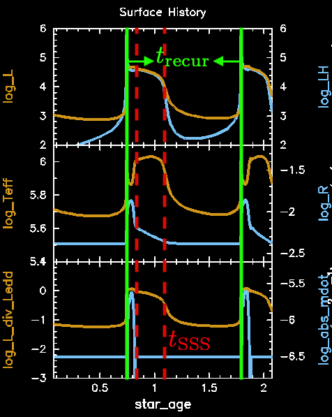
Recurrence Time: duration between successive starts of bursts
SSS Duration duration in "supersoft phase" where hydrogen-burning luminosity is very close to the photospheric luminosity
Here is a movie of a model that is clearly unstable:
And here is a movie of a model that is clearly stable:
The beginnings of flashes are the easiest to identify, so estimate the time between the two subsequent sharp rises in the luminosity to get the recurrence time.
The SSS phase duration is a little more nebulous. Estimate the the duration from the time of minimum effective temperature until the photospheric and hydrogen-burning luminosities precipitously depart from each other as they plummet.
Example estimates for the recurrence time and SSS duration for the Ṁ=3.1 × 10⁻⁷ M⊙/yr case. Here we estimate trecur=1.08 years and tSSS=0.26 yr.
Tool: Making Movies with images_to_movie
Did you check out the hint about determining stability? The videos there were composed of all the output from pgstar. In this simulation, we output a snapshot of the pgstar output with each timestep into the png directory. Take a look in there, and you'll see a png for every timestep.
To make these into a movie, the SDK comes with a nifty script that does the heavy lifting for you: images_to_movie. To use it, do something like the following:
images_to_move 'png/grid*.png' my_movie.mp4
This takes all files that match the pattern nova_grid_*.png in the png directory and then makes a movie by using each as a frame. The resulting movie is named my_movie.mp4.
You can control how often pgstar outputs pngs, what they are named, and what directory they go into in the pgstar namelist.
Warning: Stale png Directory
Before you start a new run, delete all files in png (rm -f png/*.png) or rename/move them. If you don't do this, you might end up with a mix of old and new files, and you won't know which is which.
Resolving the SSS Phase
This simulation is tuned to run quickly, and as a result, the supersoft phase doesn't last many timesteps. If we ran through it too quickly, we might actually have missed stability, while shorter timesteps might catch it. Our goal now is to modify our simulation so that it takes shorter time steps, but only during the SSS phase.
Fortunately, MESA has just the controls we want: delta_HR_limit and delta_HR_hard_limit. Both of these adjust the timestep based on how much the quantity
\[\eta = \sqrt{\left[\log (L/L_\odot)\right]^2 + \left[\log T_{\mathrm{eff}}\right]^2}\]
changes over the timestep. If η is greater than delta_HR_limit, then the next timestep will be reduced by a factor of delta_HR_limit/η. If instead η is greater than delta_HR_hard_limit, the current timestep will be retried with a shorter timestep.
We could put these in our inlist, but they will make the entire run intolerably slow. We only want really high time resolution during the SSS phase, so we will implement this in run_star_extras.f, specifically, in extras_check_model, which is executed at the end of every timestep. We want to use these tight tolerances only when the hydrogen burning luminosity is similar to the photospheric luminosity. We also only really care when the effective temperature is large.
Accessing the star info structure
Within subroutines in run_star_extras, we can access the full data in the stellar model via the "star info structure", which is usually denoted as s. All the data you can access are listed in $MESA_DIR/star/public/star_data.inc. Additionally, inlist controls are members of the star info structute, so all controls in $MESA_DIR/star/defaults/controls.defaults are can be accessed and changed.
Depending on when in the timestep you access the star info structure, some values will have already been set and/or any changes you make might be overwritten by another internal subroutine. Understanding what is set when and how often boils down to grepping around in $MESA_DIR/star/private. In extras_check_model, everything should already be set, so we don't yet need to worry about this detail (but anything we change won't affect this timestep!).
To access a member of the star info structure, we just append a % after s, followed by the name. For instance, s% mstar will return the baryonic mass of the stellar model in grams. Note that units in the star info structure are usually in cgs (unless otherwise indicated in $MESA_DIR/star/public/star_data.inc), while inlist controls are often given in solar units, so you may need to juggle conversions between the two.
Challenge: Edit extras_check_model to add a conditional that sets delta_HR_limit to 5d-3 and delta_HR_hard_limit to 1d-2 whenever LH/Lphot < 1.1 and Teff > 800,000 K and when Lphot is above the burst threshold set by L_burst. Otherwise both controls should be set to -1.
You will want to use the following in your conditional:
s% power_h_burn: total power in L⊙ produced by hydrogen burning
s% L_phot: photospheric luminosity in L⊙
s% Teff: effective temperature in Kelvin
Note that the s% means we are talking to the object that contains all the data about the stellar model, including physical quantities and inlist controls.
Use the following to set the timestep controls to the stricter limits:
s%delta_HR_limit=5d-3s%delta_HR_hard_limit=1d-2
and the looser limits:
s%delta_HR_limit=-1s%delta_HR_hard_limit=-1
The main conditional in extras_check_model should now be something like this:
! set defaults (no extra resolution)s%delta_HR_limit=-1s%delta_HR_hard_limit=-1if(s%L_phot>L_burst)thenif(waiting_for_burst)thennum_bursts=num_bursts+1write(*,2)'num_bursts',num_burstswaiting_for_burst=.false.endif! if we are in SSS, add resolutionif(s%power_h_burn/s%L_phot.LT.1.1d0.AND.s%Teff>8d5)thens%delta_HR_limit=5d-3s%delta_HR_hard_limit=1d-2endifelseif(s%L_phot<L_between)thenif(num_bursts>=2)thenwrite(*,*)'have finished burst'extras_check_model=terminates%termination_code=t_extras_check_modelendifwaiting_for_burst=.true.endif
Note that the outer conditional takes care of the luminosity condition automatically.
Challenge: Recompile and rerun your model at the same Ṁ, but now with the increased time resolution. Report the same quantities as before, but now on the second tab of the google spreadsheet.
A New Wind Scheme
The super eddington wind scheme we've been using for mass loss is simple and convenient, but you may have noticed that it continues well into the supersoft phase. In fact, this is largely due to the fact that we've moved the outer boundary condition to an optical depth of 20, which has the effect of making the model think it is super-eddington.
Let's try replacing this wind scheme with the optically-thick wind model from Kato & Hachisu 1994. They give a relatively simple law for the mass loss rate as a function of effective temperature:
\[\log\left(\dot{M}/\mathrm{g/s}\right) = -1.49 \log\left(T_{\mathrm{eff}}/10^5\,\mathrm{K}\right) + b\]
where b is a parameter that varies with the mass of the underlying white dwarf and is given by the table
This is implemented in MESA as the "nova" wind option. You can find the related controls in $MESA_DIR/star/defaults/controls.defaults.
Challenge: Edit inlist_nova [only] to deactivate the super eddington wind, and activate the nova wind. The nova wind should only be active for Teff < 3 × 10⁵ K and L > 104 L⊙. At a radius of 100 R⊙, set a Roche lobe overflow Ṁ of 10-3 M⊙/yr.
To shut off the super eddington winds, you can do one of two things to the super_eddington_scaling_factor control:
Set it to 0 (instead of 1), which multiplies any calculated wind by 0.
Comment out or delete the line. This will revert the value to its default, which is 0.
You will need to set the following controls to appropriate values:
nova_scaling_factor
nova_wind_b
nova_wind_max_Teff
nova_wind_min_L
nova_roche_lobe_radius
nova_RLO_mdot
You don't need to worry about nova_min_Teff_for_accretion yet, so don't set it.
Something like this should appear in your controls namelist:
! parameter for mass loss driven by super Eddington luminosity. Final! mdot is multiplied by this value, so 0 shuts wind off (default)super_eddington_scaling_factor=0! multiply Ledd by this factor when computing super Eddington wind! e.g., if this is 2, then only get wind when L > 2*Leddsuper_eddington_wind_Ledd_factor=1nova_scaling_factor=1! turn the wind on full blastnova_wind_b=20.77! interpolated from tablenova_wind_max_Teff=3d5! don't calculate wind if hotter than thisnova_wind_min_L=1d4! don't calculate wind if less luminous than thisnova_roche_lobe_radius=1d2! at radii above this, use `nova_RLO_mdot`nova_RLO_mdot=1d-3! mdot to use if radius is larger than roche_lobe_radius
You also could just delete the two lines about the super eddington wind.
Challenge: Rerun your model at the same Ṁ as the first two times. Now it should use the nova wind prescription and have the higher time resolution in the SSS phase. Report the same quantities as before, but now on the third tab of the google spreadsheet.
Controlling Accretion
In both wind prescriptions, if the model wasn't losing mass, it was gaining it. In reality, a nova eruption might disrupt its accretion disk or clear out a wind from a red giant donor. More practically (and less physically motivated), sometimes switching from mass gain in one timestep to mass loss in the next can create numerical difficulties. One solution is to have a buffer time in between mass loss and gain in which no mass change takes place.
You may have noticed the nova_min_Teff_for_accretion control in the last challenge. The name of this control suggests that it might be just what we want!
Challenge: Use the nova_min_Teff_for_accretion control to shut off accretion when Teff < 6 × 10⁵ K. Run the model and confirm that this worked by watching the history of Ṁ and Teff on the pgstar dashboard.
Something like this should appear in your controls namelist:
nova_min_Teff_for_accretion=6d5
Uh oh... that control didn't work, did it? The documentation in $MESA_DIR/star/defaults/controls.defaults tells us
When nova_scaling_factor /= 0 and Teff < this and L > nova_wind_min_L, no accretion. That sure sounds right, so what's going on? Have we found a bug?
Let's take a look at the source to see where this control actually comes in to play. Most of the good sciency bits of code are found in $MESA_DIR/star/private. The functions and subroutines there aren't accessible to you in run_star_extras.f, but they can help you see how the sausage is made.
Challenge: Look in $MESA_DIR/star/private to find where nova_min_Teff_for_accretion is implemented.
To search for "example" in all fortran (.f90) files in $MESA_DIR/star/private, try using grep:
cd $MESA_DIR/star/private grep "example" *.f90
First, to find the relevant lines, we do cd $MESA_DIR/star/private grep "nova_min_Teff_for_accretion" *.f90
We then get the following output (in mesa revision 11701):
All but the last are code that just deal with defining and loading valid controls from namelists. So the implementation is in winds.f90. There we find that it's thrown away in a comment!
Perhaps you can see the problem. If T1 (which here is the surface temperature) is less than the paramter, it will always set the change in the star's mass to be zero. That is, not only will mass gain be turned off, but so is our wind.
So it looks like the original implementation of this control didn't really work as intended. (Aside: this was discovered, and the quick fix was to deactivate the control, but then the real fix has not yet been committed). So we're going to implement it!
To implement this control, we'll use one of MESA's "other" hooks, prototyped in $MESA_DIR/star/other. These files each allow you to drop some code into your run_star_extras.f that are injected into the evolution at runtime. The proper one to use here is other_adjust_mdot, which gives us the last word on mass gain or loss in the star (by ultimately setting s% mstar_dot).
Setting Up A Null Hook
Before we implement this control, let's set up a hook into MESA that does nothing but print a statement out to the terminal so we know it's being called. Copy the null_other_adjust_mdot subroutine from $MESA_DIR/star/other/other_adjust_mdot.f90 into src/run_star_extras in your local nova directory, right below end subroutine extras_controls. Rename the subroutine something more descriptive, like nova_adjust_mdot (be sure to update the name at the beginning and the end of the subroutine).
Just because the subroutine is there doesn't mean it will be called when MESA is checking for the other_adjust_mdot hook. We need to edit extras_conrols to tell it that our new subroutine should be injected at that stage of evolution by adding
s%other_adjust_mdot=>nova_adjust_mdot
The two subroutines together should now look like this:
subroutineextras_controls(id,ierr)integer,intent(in)::idinteger,intent(out)::ierrtype(star_info),pointer::sierr=0callstar_ptr(id,s,ierr)if(ierr/=0)returns%extras_startup=>extras_startups%extras_check_model=>extras_check_models%extras_finish_step=>extras_finish_steps%extras_after_evolve=>extras_after_evolves%how_many_extra_history_columns=>how_many_extra_history_columnss%data_for_extra_history_columns=>data_for_extra_history_columnss%how_many_extra_profile_columns=>how_many_extra_profile_columnss%data_for_extra_profile_columns=>data_for_extra_profile_columns! YOU ADDED THIS LINEs%other_adjust_mdot=>nova_adjust_mdotendsubroutineextras_controlssubroutinenova_adjust_mdot(id,ierr)usestar_definteger,intent(in)::idinteger,intent(out)::ierrierr=0endsubroutinenova_adjust_mdot
Now let's add our write statement into nova_adjust_mdot, right after ierr = 0:
subroutinenova_adjust_mdot(id,ierr)usestar_definteger,intent(in)::idinteger,intent(out)::ierrierr=0write(*,*)"Hello from nova_adjust_mdot!"endsubroutinenova_adjust_mdot
Compile your code to make sure there aren't any syntax errors with ./mk. Assuming things compiled fine, there's one last step you need to do to make MESA actually call our subroutine: add the line use_other_adjust_mdot = .true. to the controls namelist. After you've done that, run the simulation to see if your friendly message shows up at every timestep.
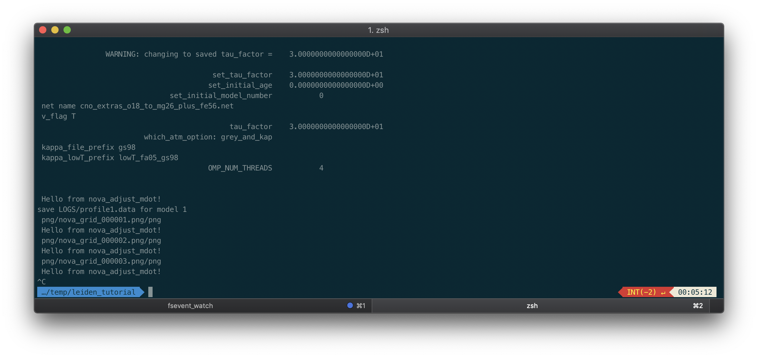
Output with our pointless other_adjust_mdot properly working.
Now we are almost ready to do something interesting. Delete the write statement from your subroutine. We need to get access to the star info structure, which is the entity that lets us access and change physical details about the star. Each stellar model has an integer id. We can get the star info structure loaded by using this id, which is the main argument to our subroutine. You'll need to add two lines to your subroutine:
type (star_info), pointer :: s: put this line before the ierr = 0 line, since all declarations must come at the beginning of a subroutine; this line allocates space for the star info structure and names it s, which is a common convention throughout MESA
call star_ptr(id, s, ierr): this conjures up the star info structure into s from the id provided in the signature to our subroutine. Now we can use s as a handle into our stellar model. Put it after ierr = 0
Double check that your code compiles. If it does, now you're ready to actually implement this control!
Challenge: Finish the implementation of nova_adjust_mdot. Set s% mstar_dot = 0d0 if all of the following conditions are met simultaneously:
Value set by nova_scaling_factor > 0
Luminosity is above value set by nova_wind_min_L
Effective temperature is in between values set by nova_wind_max_Teff and nova_min_Teff_for_accretion
Otherwise, it should do nothing.
You'll want to make use of the following members of the star info structure (that are just taken from the controls namelist):
nova_scaling_factor
nova_nova_wind_min_L (note that this is in L⊙)
nova_wind_max_Teff
nova_min_Teff_for_accretion
and the following from the model's physical data (found in $MESA_DIR/star/public/star_data.inc):
mstar_dot
Teff
L_phot (fortunately, this is also in L⊙, so we don't need to convert)
Your full implementation of nova_adjust_mdot should look something like this:
We didn't need to worry about this in this exercise, but often quantities are stored in the star info structure in cgs, but relevant controls (and indeed some of the internal values in the star info structure) are expressed in solar units. Converting between these (and many other tasks) are made easy by the const module, whidh is loaded at the top of your run_star_extras.f file:
usestar_libusestar_defuseconst_def! loads all sorts of goodies
Look in $MESA_DIR/const/public/const_def.f90 to see what constants are already available. So long as the module is loaded, you don't need to declare these or anything before using them, and they aren't part of the star info structure, so you could just reference Lsun directly in any of the code, and it will evaluate to a solar luminosity in cgs.
Challenge: Rerun your model at the same Ṁ as the first three times. Now it should use the nova wind prescription with the higher time resolution in the SSS phase and accretion should stop before mass loss begins (if it ever begins). Report the same quantities as before, but now on the fourth tab of the google spreadsheet.
Discussion
You should find that mass loss doesn't even occur anymore; simply stopping accretion halts the redward surge before the nova wind can begin. As a result, recurrence times and SSS phase durations should increase. You could simulate different scenarios where accretion resumes at later and later times by increasing nova_min_Teff_for_accretion, perhaps even setting it to something ludicrously high, like 107 K, so that no accretion ever happens during the SSS phase. In this case, we wouldn't expect there to be any Ṁ with stable burning (what Kato & Hachisu call "enforced novae").
The super eddington wind prescription, in additon to being poorly resolved in time, suffered from mass loss continuing well into the SSS phase, which if we dug deeper, we would realize would not happen had we not set our surface boundary condition at τ=20. We still haven't touched on what changing the spatial resolution would do, or more importantly how convective boundary mixing during the runaway would change things. There are still many experiments to run!